Class 11 Economics Book 2 Ch 2 Notes: Theory of Consumer Behaviour

Covers T.R. Jain & V.K. Ohri (2026-27) ch 3-6. Based on NCERT Introductory Microeconomics, Chapter 2 (Reprint 2026-27), the CBSE curriculum 2026-27 (Unit 5, 14 marks) and the CBSE Supplementary Reading Material.

Board note: CBSE teaches this book in Class 11; UP, Bihar, Rajasthan and MP Boards teach it in Class 12 Microeconomics.

In this chapter you will learn to

work out total and marginal utility and explain the law of diminishing marginal utility
find the consumer’s equilibrium by utility analysis (MU = P and MUx/Px = MUy/Py)
explain the indifference curve, MRS, the indifference map and the features of indifference curves
write the budget set and budget line, its equation and slope, and show how it moves when income or a price changes
locate the consumer’s optimum at the point of tangency (MRS = p1/p2)
explain demand, the law of demand, derivation of the demand curve, movement and shift, and market demand
measure price elasticity of demand by the percentage method, on a linear curve and by the total expenditure method

utilitytotal utilitymarginal utilitycardinalordinalconsumption bundleindifference curvemarginal rate of substitutionmonotonic preferencesindifference mapbudget setbudget linebudget constraintrational consumeroptimum bundledemand functionlaw of demandsubstitution effectincome effectnormal goodinferior goodGiffen goodsubstitutescomplementsmarket demandhorizontal summationprice elasticity of demandrectangular hyperbola

1 The problem of choice and basic notation

Every consumer has to decide how to spend her income on different goods; economists call this the problem of choice
She wants the combination that gives her maximum satisfaction; this ‘best’ combination depends on two things:
- the consumer’s likes, also called preferences
- what she can afford, which depends on the prices of the goods and her income
Two approaches explain consumer behaviour: (i) Cardinal Utility Analysis and (ii) Ordinal Utility Analysis
In the book, “goods” means goods as well as services

Preliminary notations and assumptions

For simplicity there are only two goods: bananas and mangoes; this lets simple diagrams explain the ideas
Any combination of amounts of the two goods is a consumption bundle, or simply a bundle
$x_1$ = quantity of bananas, $x_2$ = quantity of mangoes; both can be positive or zero
$(x_1, x_2)$ is the bundle with $x_1$ bananas and $x_2$ mangoes. So (5, 10) has 5 bananas and 10 mangoes, while (10, 5) has 10 bananas and 5 mangoes

2 Utility

Learn by heartDefinition 1

Utility of a commodity is its want-satisfying capacity. The stronger the need for a commodity or the desire to have it, the greater the utility derived from it.

Subjective

Different people get different utility from the same commodity. Someone who likes chocolates gets much higher utility from a chocolate

Changes with place

The utility of a room heater depends on whether the person is in Ladakh or in Chennai

Changes with time

The same room heater is more useful in winter than in summer

3 Cardinal utility analysis

Learn by heartDefinition 2

Cardinal utility analysis assumes that the level of utility can be expressed in numbers. For example: “this shirt gives me 50 units of utility”.

3.1 Two measures of utility

Learn by heartDefinition 3

Total utility (TU) of a fixed quantity of a commodity is the total satisfaction derived from consuming that amount of commodity x. More of x gives more satisfaction, so TU depends on the quantity consumed. $TU_n$ = total utility from n units of x.

Learn by heartDefinition 4

Marginal utility (MU) is the change in total utility due to the consumption of one additional unit of a commodity: $MU_n = TU_n – TU_{n-1}$

Book example

4 bananas give 28 units of total utility and 5 bananas give 30 units
The 5th banana raised total utility by 2 units: $MU_5 = TU_5 – TU_4 = 30 – 28 = 2$

How TU and MU are related

MU_n = TU_n – TU_{n-1} \qquad TU_n = MU_1 + MU_2 + \dots + MU_{n-1} + MU_n

So the total utility of n units is the sum of the marginal utilities of each unit.

3.2 Table 2.1 and the law of diminishing marginal utility

Units	Total utility (TU)	Marginal utility (MU)	What is happening
1	12	12	TU rises, but at a diminishing rate; MU falls
2	18	18 − 12 = 6
3	22	22 − 18 = 4
4	24	24 − 22 = 2
5	24	24 − 24 = 0	TU at its maximum (constant), MU zero
6	22	22 − 24 = −2	TU starts falling, MU negative

The book’s Table 2.1 (an imaginary example). MU diminishes from 12 to 6, 6 to 4 and so on.

Figure 1: From Table 2.1: total utility is highest (24) at the 5th unit, where marginal utility is zero; at the 6th unit MU is negative (−2) and TU falls to 22 — **Figure 1**: From Table 2.1: total utility is highest (24) at the 5th unit, where marginal utility is zero; at the 6th unit MU is negative (−2) and TU falls to 22

Learn by heartDefinition 5

Law of Diminishing Marginal Utility: marginal utility from consuming each additional unit of a commodity declines as its consumption increases, while keeping consumption of other commodities constant.

Reason: having obtained some amount of the commodity, the consumer’s desire to have still more of it becomes weaker
MU becomes zero at the level where TU remains constant (the 5th unit in the table)
After that TU starts falling and MU becomes negative

Position of MU	Behaviour of TU
MU positive but falling	TU rises at a diminishing rate
MU = 0	TU at its maximum (highest point)
MU negative	TU falls

Worked example 1: MU from TU (CBSE supplementary material’s table)

Q. Total utility from 1 to 6 units of a good is 4, 7, 9, 10, 10, 9. Find marginal utility and name the law it shows.

Formula: $MU_n = TU_n – TU_{n-1}$ (½)
MU: 4 (= 4 − 0), 3 (= 7 − 4), 2 (= 9 − 7), 1 (= 10 − 9), 0 (= 10 − 10), −1 (= 9 − 10) (1)
Each further unit’s MU is lower than the previous one: law of diminishing marginal utility (½)
Meaning: TU is highest (10) at the 5th unit because MU = 0 there; the 6th unit reduces satisfaction

Common mistakes

MU of the first unit equals TU of the first unit (here $TU_0 = 0$ ); leaving it blank is wrong
“TU is maximum when MU is maximum” is wrong; TU is maximum when MU = 0
MU can be negative while TU is still positive (6th unit in the table: TU 22, MU −2)

3.3 Derivation of the demand curve for a single commodity

Learn by heartDefinition 6

Demand: the quantity of a commodity that a consumer is willing to buy and is able to afford, given the prices of goods and the income of the consumer, is called demand for that commodity.

Demand for commodity x depends, apart from its own price, on the prices of other commodities (substitutes and complements), the income of the consumer and her tastes and preferences
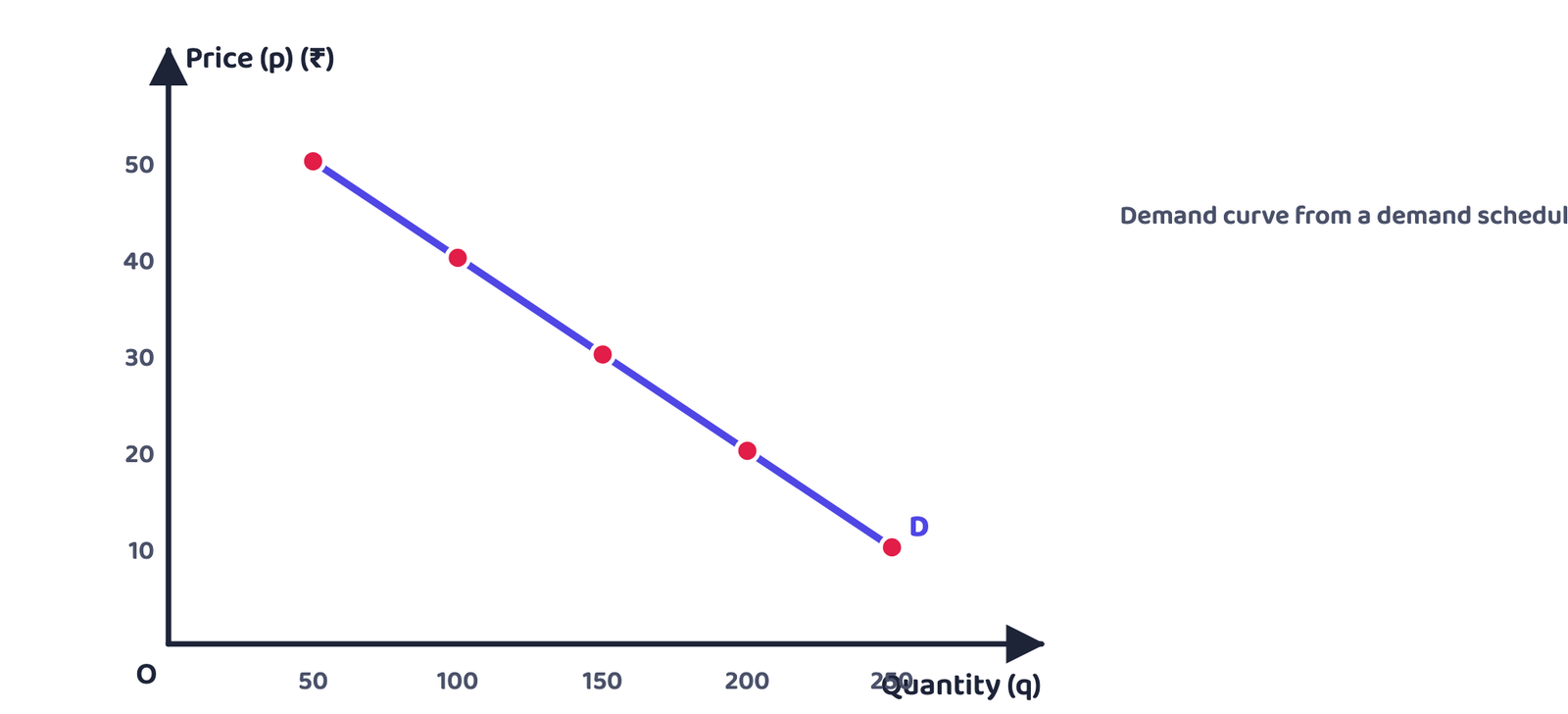
The demand curve is a graph of the quantities a consumer is willing to buy at different prices of the commodity, holding constant the prices of related commodities and income
Quantity is measured on the horizontal axis and price on the vertical axis; the curve slopes downward: more is bought at lower prices, less at higher prices
This negative relationship between price and quantity demanded is the Law of Demand

1Each successive unit gives lower marginal utility (diminishing MU)

↓

2So the consumer is not willing to pay as much for each additional unit

↓

3At ₹40 per unit she demands 5 units; the 6th unit is worth less than the 5th, so she buys it only when the price drops below ₹40

↓

4The demand curve slopes downward (negative slope)

3.4 Consumer’s equilibrium by utility analysis

This part is in the CBSE curriculum 2026-27 (“conditions of consumer’s equilibrium using marginal utility analysis”) and is taken from the CBSE Supplementary Reading Material; the rationalised NCERT text does not give it separately.

Learn by heartDefinition 7

Consumer’s equilibrium is the situation in which the consumer, with given income and prices, spends in such a way that she gets maximum satisfaction and has no reason to change her spending.

(a) One good: MU = P

Take utility as measured in rupees; the consumer compares the MU of each unit with its price (P)
While MU > P, buying a unit pays (she gets more than she gives); as she buys more, MU falls
She stops where MU = P; beyond that MU < P and the next unit is a losing bargain

Unit	Price (₹)	MU (₹)	Decision
1	3	8	MU > P, buy
2	3	7	MU > P, buy
3	3	5	MU > P, buy
4	3	3	MU = P, equilibrium
5	3	2	MU < P, will not buy

Example from the CBSE Supplementary Reading Material: the consumer maximises satisfaction by buying 4 units.

Figure 2: Equilibrium with one good (CBSE supplementary material): at a price of ₹3 the consumer buys 4 units, where MU = P (point E) — **Figure 2**: Equilibrium with one good (CBSE supplementary material): at a price of ₹3 the consumer buys 4 units, where MU = P (point E)

(b) Two goods: equi-marginal utility

The consumer buys two goods X and Y with given income and prices $P_x$ , $P_y$ . There are two conditions of equilibrium:

Conditions of equilibrium with two goods

\frac{MU_x}{P_x} = \frac{MU_y}{P_y} = \text{MU of a rupee}

Condition 1: the marginal utility from the last rupee spent on each good is the same (also called the Law of Equi-Marginal Utility). Condition 2: MU of a good falls as more of it is consumed (diminishing MU).

Suppose $\dfrac{MU_x}{P_x} \gt \dfrac{MU_y}{P_y}$ : a rupee spent on X gives more utility than a rupee spent on Y
The consumer moves a rupee from Y to X: she gains more utility than she loses
Buying more X lowers $MU_x$ , buying less Y raises $MU_y$ ; this goes on until the two ratios are equal
Without condition 2 (MU not falling) the ratios might never be equal and the consumer would end up buying just one good

Worked example 2: equilibrium with two goods

Q. Income ₹15, $P_x$ = ₹2, $P_y$ = ₹3. MU of the first 5 units of X: 20, 16, 12, 8, 4; of Y: 30, 24, 18, 12, 6. Find the equilibrium bundle.

Unit	MUx	MUx/Px	MUy	MUy/Py
1	20	10	30	10
2	16	8	24	8
3	12	6	18	6
4	8	4	12	4
5	4	2	6	2

Condition: $\dfrac{MU_x}{P_x} = \dfrac{MU_y}{P_y}$ with the whole income spent (½)
At 3 units of X and 3 units of Y both ratios are 6; spending = 2 × 3 + 3 × 3 = ₹15 = income (1)
Equilibrium bundle: X = 3, Y = 3; total utility = (20 + 16 + 12) + (30 + 24 + 18) = 120 (½)
Meaning: the last rupee on each good gives the same utility (6); no other bundle costing ₹15 gives more than 120

The law of demand from utility

In equilibrium $\dfrac{MU_x}{P_x} = \dfrac{MU_y}{P_y}$ . If $P_x$ falls, $\dfrac{MU_x}{P_x} \gt \dfrac{MU_y}{P_y}$
The consumer buys more X and less Y until $MU_x$ falls and the ratios are equal again
With one good too: if price falls, MU > P, so she buys more units
Either way, when price falls, demand rises: the law of demand

4 Ordinal utility analysis

Cardinal analysis is simple to understand but has a major drawback: quantification of utility in numbers
In real life we never express utility in numbers; at most we rank combinations as having more or less utility
The consumer does not measure utility but she ranks bundles; this is the starting point of ordinal utility analysis

Learn by heartDefinition 8

Ordinal utility analysis does not measure utility in numbers; it only ranks bundles in order of more or less satisfaction.

4.1 Indifference curve

Learn by heartDefinition 9

An indifference curve (IC) joins all points representing bundles among which the consumer is indifferent, that is, bundles that give her equal satisfaction.

All points such as A, B, C and D on an indifference curve give the same level of satisfaction
To get one more banana and stay on the same curve (same satisfaction), the consumer must give up some mangoes; so the curve slopes downward

Learn by heartDefinition 10

The marginal rate of substitution (MRS) is the amount of mangoes the consumer has to forego to get an additional banana, her total utility being the same. It is the rate at which she substitutes bananas for mangoes: $MRS = \left|\dfrac{\Delta Y}{\Delta X}\right|$

MRS is only the magnitude (absolute value) of $\Delta Y/\Delta X$ : if $\Delta Y/\Delta X = -3/1$ , MRS = 3

Combination	Quantity of bananas (Qx)	Quantity of mangoes (Qy)	MRS
A	1	15	–
B	2	12	3 : 1
C	3	10	2 : 1
D	4	9	1 : 1

The book’s Table 2.2: representation of the law of diminishing marginal rate of substitution.

Figure 3: Indifference curve through A, B, C and D of Table 2.2: the mangoes given up for each extra banana fall 3, 2, 1 (diminishing MRS), so the curve is convex to the origin — **Figure 3**: Indifference curve through A, B, C and D of Table 2.2: the mangoes given up for each extra banana fall 3, 2, 1 (diminishing MRS), so the curve is convex to the origin

Learn by heartDefinition 11

Law of Diminishing Marginal Rate of Substitution: as the quantity of bananas increases, the quantity of mangoes sacrificed for each additional banana (MRS) declines.

A to B: 3 mangoes for 1 banana; B to C: 2 mangoes; C to D: just 1 mango
Reason: as bananas increase, the MU from each additional banana falls; as mangoes fall, the MU of mangoes rises; so the consumer is inclined to sacrifice smaller and smaller amounts of mangoes

4.2 Shape of an indifference curve

The law of diminishing MRS makes an indifference curve convex to the origin; this is the most common shape
For perfect substitutes the MRS does not diminish; it stays constant, so the indifference curve is a straight line

Learn by heartDefinition 12

Perfect substitutes are goods that can be used in place of each other and give exactly the same level of utility to the consumer.

Combination	Five-rupee notes	Five-rupee coins	MRS
A	1	8	–
B	2	7	1 : 1
C	3	6	1 : 1
D	4	5	1 : 1

The book’s Table 2.3. As long as the total of notes and coins stays the same (9), the consumer is indifferent; a ₹5 coin and a ₹5 note are the same to her.

Figure 4: Perfect substitutes (Table 2.3): ₹5 notes and coins; MRS is always 1 : 1, so the indifference curve is a straight line — **Figure 4**: Perfect substitutes (Table 2.3): ₹5 notes and coins; MRS is always 1 : 1, so the indifference curve is a straight line

4.3 Monotonic preferences

Learn by heartDefinition 13

Monotonic preferences: between any two bundles $(x_1, x_2)$ and $(y_1, y_2)$ , if $(x_1, x_2)$ has more of at least one good and no less of the other, the consumer prefers $(x_1, x_2)$ . Preferences of this kind are called monotonic.

Quick check

(10, 8) vs (8, 6): the first has more of both goods, so a consumer with monotonic preferences prefers (10, 8); she cannot be indifferent between them
(6, 6) vs (5, 6): the first has more bananas and the same mangoes; a monotonic consumer chooses (6, 6)

4.4 Indifference map

Learn by heartDefinition 14

An indifference map is a family of indifference curves representing the consumer’s preferences over all bundles. Monotonicity means that between any two curves the bundles on the higher one are preferred to those on the lower one.

Figure 5: A family of indifference curves IC₁, IC₂, IC₃; the arrow shows the direction of higher satisfaction; points A, B, C are from Table 2.4 (feature 2 below) — **Figure 5**: A family of indifference curves IC₁, IC₂, IC₃; the arrow shows the direction of higher satisfaction; points A, B, C are from Table 2.4 (feature 2 below)

4.5 Features of indifference curves

The book lists three features (1-3); the fourth point, convexity, comes from section 4.2 “Shape of an indifference curve”.

Slopes downward from left to right

More bananas mean giving up some mangoes. If no mangoes were given up, the consumer would have more bananas and the same mangoes and be on a higher curve. So on the same curve: $\Delta x_1 \gt 0$ means $\Delta x_2 \lt 0$

Higher curve, higher utility

As long as MU is positive, more of a good gives more satisfaction. Combinations with more mangoes, more bananas or more of both lie on higher curves

Two curves never intersect

Intersecting curves would lead to conflicting results

Shape: convex to the origin

See section 4.2

Proof of feature 2: Table 2.4

Combination	Quantity of bananas	Quantity of mangoes
A	1	10
B	2	10
C	3	10

All three have the same mangoes (10); B has more bananas than A, so B gives more satisfaction and lies on a higher curve
C has more bananas than B, so C lies on a curve higher still (in the figure above A, B and C lie on IC₁, IC₂ and IC₃)

Proof of feature 3: Figure 2.8 of the book

Figure 6: Two indifference curves cannot intersect (book Fig. 2.8): A and B on IC₁, A and C on IC₂; B and C would then give equal satisfaction although B has more mangoes — **Figure 6**: Two indifference curves cannot intersect (book Fig. 2.8): A and B on IC₁, A and C on IC₂; B and C would then give equal satisfaction although B has more mangoes

A (7, 10) and B (9, 7) lie on the same curve IC₁so A and B give equal satisfaction

A (7, 10) and C (9, 5) lie on the same curve IC₂so A and C give equal satisfaction

Then B and C also give equal satisfactionboth equal A

But B has the same bananas (9) and more mangoes (7 > 5)with monotonic preferences B is better: an absurd result

So two indifference curves cannot intersectthe assumption of intersection is disproved

Basis	Cardinal utility	Ordinal utility
Measurement	In numbers (50 units)	Only ranking (more/less)
Main tools	TU, MU, diminishing MU	Indifference curves, MRS, budget line
Equilibrium condition	MUx/Px = MUy/Py	MRS = Px/Py, IC convex
Merit/drawback	Simple, but counting utility is unrealistic	More realistic; needs only ranking

Utility function

The book’s summary says that, besides an indifference map, a consumer’s preferences can also be represented by a utility function. A utility function gives each bundle a number such that a preferred bundle gets a larger number; all bundles on one indifference curve get the same number.

5 The consumer’s budget

The consumer has a fixed income to spend on two goods, and the prices are given in the market
She cannot buy every combination she wants; only bundles that cost less than or equal to her income

5.1 Budget set and budget line

Income = M; prices of bananas and mangoes = $p_1$ and $p_2$
The price of a good is the amount of money the consumer has to pay per unit of the good she wants to buy (a banana price of $p_1$ means $p_1$ rupees per kilogram)
Spending on $x_1$ bananas is $p_1x_1$ , on $x_2$ mangoes $p_2x_2$ ; the bundle costs $p_1x_1 + p_2x_2$

Learn by heartDefinition 15

Budget constraint: the consumer can buy any bundle $(x_1, x_2)$ such that $p_1x_1 + p_2x_2 \le M$ …(2.1). This inequality is the consumer’s budget constraint.

Learn by heartDefinition 16

The budget set is the collection of all bundles that the consumer can buy with her income at the prevailing market prices.

Book’s Example 2.1: integer units

Income ₹20; both goods priced at ₹5; available only in whole units; condition $5x_1 + 5x_2 \le 20$ , that is $x_1 + x_2 \le 4$
The 15 affordable bundles: (0,0), (0,1), (0,2), (0,3), (0,4), (1,0), (1,1), (1,2), (1,3), (2,0), (2,1), (2,2), (3,0), (3,1), (4,0)
Of these, 5 cost exactly ₹20: (0,4), (1,3), (2,2), (3,1), (4,0); the other 10 cost less than ₹20
(3,3) costs ₹30 and (4,5) costs ₹45; these exceed ₹20 and cannot be bought

Figure 7: Budget set of Example 2.1: income ₹20, both prices ₹5; 15 bundles are affordable, 5 of them on the budget line x₁ + x₂ = 4 (exactly ₹20) — **Figure 7**: Budget set of Example 2.1: income ₹20, both prices ₹5; 15 bundles are affordable, 5 of them on the budget line x₁ + x₂ = 4 (exactly ₹20)

If the goods are perfectly divisible (you can buy half a kilogram of rice or one-fourth of a litre of milk, but not half an orange or one-fourth of a banana), the budget set is every point in the positive quadrant on or below the line

Learn by heartDefinition 17

The budget line consists of all bundles that cost exactly M (the whole income): $p_1x_1 + p_2x_2 = M$ …(2.2). Points below the budget line are bundles that cost strictly less than M.

Budget line formulas

x_2 = \frac{M}{p_2} – \frac{p_1}{p_2}x_1 \qquad (2.3)

\text{horizontal intercept} = \frac{M}{p_1} \qquad \text{vertical intercept} = \frac{M}{p_2} \qquad \text{slope} = -\frac{p_1}{p_2}

(2.3) has the form of the straight line

y = c + mx

(c the vertical intercept, m the slope). The horizontal intercept is the bundle with the whole income spent on bananas; the vertical intercept, on mangoes.

5.2 Price ratio and the slope of the budget line

Every point on the budget line uses up the whole budget; one more banana is possible only by giving up some of the other good
A banana costs $p_1$ , so spending on mangoes must fall by $p_1$ ; with $p_1$ she could buy $p_1/p_2$ mangoes
So one extra banana costs $p_1/p_2$ mangoes: in the market she can substitute bananas for mangoes at the rate $p_1/p_2$
The absolute value of the budget line’s slope is the rate at which she is able to substitute bananas for mangoes while spending her whole budget (the absolute value $|x|$ is x if x ≥ 0 and −x if x < 0)

Derivation of the slope of the budget line

p_1x_1 + p_2x_2 = M

…(2.4)a point

(x_1, x_2)

on the budget line

p_1(x_1 + \Delta x_1) + p_2(x_2 + \Delta x_2) = M

…(2.5)another point on the same line (∆ = “a change”)

p_1\Delta x_1 + p_2\Delta x_2 = 0

…(2.6)subtracting (2.4) from (2.5)

\dfrac{\Delta x_2}{\Delta x_1} = -\dfrac{p_1}{p_2}

…(2.7)rearranging terms

Worked example 3: budget line

Q. Income ₹60, price of bananas ₹5, price of mangoes ₹3. Write the budget line, both intercepts and the slope.

Given

M = 60, $p_1$ = 5, $p_2$ = 3

To find

equation, intercepts, slope

Equation: $5x_1 + 3x_2 = 60$ (1)
Whole income on bananas: $M/p_1 = 60/5 =$ 12 bananas; on mangoes: $M/p_2 = 60/3 =$ 20 mangoes (1)
Slope $= -p_1/p_2 =$ −5/3 (1)
Meaning: spending the whole budget, one more banana costs 5/3 (about 1.67) mangoes

5.3 Changes in the budget set

(a) A change in income (prices constant)

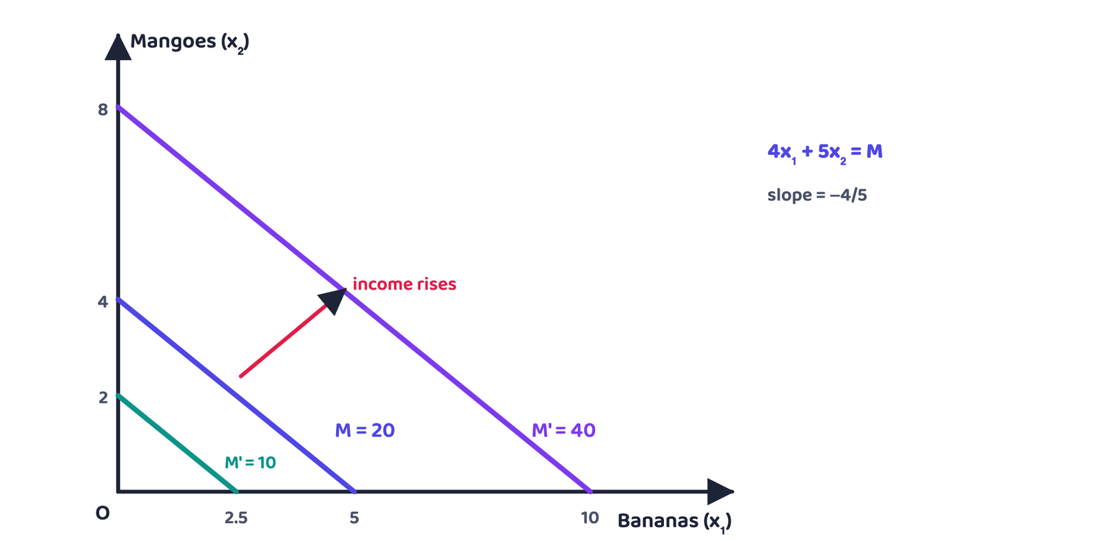
Income changes from M to M′: new line $p_1x_1 + p_2x_2 = M'$ …(2.8), that is $x_2 = \dfrac{M'}{p_2} – \dfrac{p_1}{p_2}x_1$ …(2.9)
The slope is unchanged ( $-p_1/p_2$ ) but the intercepts change
M′ > M: both intercepts rise, a parallel outward shift of the budget line; she can buy more of the goods
M′ < M: both intercepts fall, a parallel inward shift; availability of goods goes down

Figure 8: Change in income (p₁ = 4, p₂ = 5): at incomes 10, 20 and 40 the budget line shifts parallel; intercepts 2.5 and 2, 5 and 4, 10 and 8 — **Figure 8**: Change in income (p₁ = 4, p₂ = 5): at incomes 10, 20 and 40 the budget line shifts parallel; intercepts 2.5 and 2, 5 and 4, 10 and 8

(b) A change in the price of one good (income and the other price constant)

Price of bananas changes from $p_1$ to $p'_1$ : $p'_1x_1 + p_2x_2 = M$ …(2.10), that is $x_2 = \dfrac{M}{p_2} – \dfrac{p'_1}{p_2}x_1$ …(2.11)
The vertical intercept is unchanged ( $M/p_2$ ); the slope and horizontal intercept change
$p'_1 \gt p_1$ : the absolute slope rises, the line becomes steeper (it pivots inwards around the vertical intercept and the horizontal intercept falls)
$p'_1 \lt p_1$ : the line becomes flatter (it pivots outwards and the horizontal intercept rises)
A change in the price of mangoes works the same way, but now the horizontal intercept stays and the line pivots around it

Figure 9: Change in the price of bananas (M = 20, p₂ = 5): the vertical intercept 4 stays; the line becomes steeper when p₁ rises from 4 to 5 and flatter when it falls from 4 to 2 — **Figure 9**: Change in the price of bananas (M = 20, p₂ = 5): the vertical intercept 4 stays; the line becomes steeper when p₁ rises from 4 to 5 and flatter when it falls from 4 to 2

Change	Slope	What stays fixed	Behaviour of the line
Income rises	Same	Prices	Parallel outward
Income falls	Same	Prices	Parallel inward
$p_1$ rises	Steeper	Vertical intercept	Horizontal intercept moves in
$p_1$ falls	Flatter	Vertical intercept	Horizontal intercept moves out
$p_2$ falls	Flatter	Horizontal intercept	Vertical intercept moves up
Income and both prices double	Same	All ratios	No change

Common mistakes

Writing the slope as $-p_2/p_1$ is wrong; the price of the good on the horizontal axis (good 1) goes on top: $-p_1/p_2$
Writing the horizontal intercept as $M/p_2$ is wrong; good 1 is on the horizontal axis, so it is $M/p_1$
When income changes the line does not “pivot”; it shifts parallel. Pivoting happens when a price changes

Basis	Budget set	Budget line
Meaning	All affordable bundles	Only bundles that use up the whole income
Condition	$p_1x_1 + p_2x_2 \le M$	$p_1x_1 + p_2x_2 = M$
In the diagram	The whole area on and below the line	Only the line

6 Optimal choice of the consumer

The consumer chooses from the budget set on the basis of her tastes and preferences; her preferences are well defined: between any two bundles she either prefers one or is indifferent

Learn by heartDefinition 18

A rational consumer clearly knows what is good or bad for her and in any situation always tries to achieve the best for herself. From the bundles available to her she always chooses the one that gives her maximum satisfaction.

The consumer’s problem: to move to a point on the highest possible indifference curve given her budget set

6.1 Why the optimum lies on the budget line

BelowCompared with a point below the budget line, there is always a point on the line with more of at least one good and no less of the other; a monotonic consumer prefers it

↓

AbovePoints above the budget line are not available (too costly)

↓

SoThe optimum (most preferred) bundle is on the budget line

6.2 Tangency: MRS = price ratio

The optimum on the budget line is where the budget line just touches (is tangent to) one of the indifference curves
Any other point on the budget line lies on a lower indifference curve and is inferior
At the point of tangency the absolute slope of the indifference curve (MRS) equals the absolute slope of the budget line (price ratio $p_1/p_2$ )
MRS is the rate at which the consumer is willing to substitute; the price ratio is the rate at which she is able to substitute in the market; at the optimum the two are equal

Figure 10: Consumer's optimum: the budget line 4x₁ + 5x₂ = 20 is tangent to IC₂ at E (2.5, 2), where MRS = p₁/p₂ = 0.8 — **Figure 10**: Consumer’s optimum: the budget line 4x₁ + 5x₂ = 20 is tangent to IC₂ at E (2.5, 2), where MRS = p₁/p₂ = 0.8

The curve that just touches the budget line (IC₂) is the highest curve the budget set allows; bundles on higher curves (IC₃) are not affordable; bundles on lower curves (IC₁) are certainly inferior
In the figure the budget line is $4x_1 + 5x_2 = 20$ ; at E, $x_1^* = 2.5$ , $x_2^* = 2$ and spending is $4(2.5) + 5(2) = 20$ ; MRS there is 4/5 = 0.8

If MRS ≠ price ratio (the book’s argument)

Suppose at some point MRS = 2 and the two goods have the same price ( $p_1/p_2 = 1$ )
The consumer is willing to give up 2 mangoes for an extra banana, but in the market she gets a banana for just 1 mango
By buying an extra banana she can have more of both goods than before and move to a preferred bundle; so a point with MRS > price ratio is not the optimum
A similar argument holds where MRS < price ratio: she would buy fewer bananas and more mangoes

Conditions of equilibrium in indifference curve analysis

MRS_{xy} = \frac{p_1}{p_2} \quad (\text{the budget line is tangent to an IC})

Second condition: MRS must be falling at the equilibrium point, that is, the indifference curve is convex to the origin; only then does the tangency point give the highest satisfaction. The bundle also lies on the budget line (whole income spent).

The book’s footnote 9: in some situations the optimum can be at a point where the consumer spends her entire income on one of the goods only.

7 Demand

The amount of a good the consumer chooses optimally depends on: the price of the good itself, the prices of other goods, the consumer’s income and her tastes and preferences (these are the determinants of demand)
If any of these changes, the chosen quantity is likely to change; so we change one variable at a time

7.1 Demand function, demand schedule and demand curve

Learn by heartDefinition 19

Demand function: if the prices of other goods, income and tastes stay unchanged, the amount of a good the consumer optimally chooses depends entirely on its price. This relation is the demand function: $X = f(P)$ …(2.12), where X is the quantity and P the price.

What a function is (the book’s box)

A function $y = f(x)$ is a relation between x and y such that for each value of x there is a unique value of y; x is the independent variable, y the dependent variable
Example 1: x = 0, 1, 2, 3 with y = 10, 15, 18, 20; algebraic examples: $y = 5 + x$ and $y = 50 – x$
Increasing function: y does not decrease as x rises ( $y = 5 + x$ , graph slopes upward); decreasing function: y does not increase as x rises ( $y = 50 – x$ , graph slopes downward)
Usually the independent variable goes on the horizontal axis, but in the demand curve it is the opposite: the independent variable (price) is on the vertical axis and the dependent variable (quantity) on the horizontal axis

Learn by heartDefinition 20

A demand schedule is a table showing the different quantities of a good that buyers are willing to buy at different prices during a given period. The demand curve is the graphical representation of the demand function (or schedule).

Price (₹ per unit)	50	40	30	20	10
Quantity demanded (units)	50	100	150	200	250

Demand schedule from the CBSE Supplementary Reading Material: more is purchased as price falls.

Figure 11: Downward sloping demand curve drawn from the CBSE supplementary material's demand schedule (50 units at ₹50 to 250 units at ₹10) — **Figure 11**: Downward sloping demand curve drawn from the CBSE supplementary material’s demand schedule (50 units at ₹50 to 250 units at ₹10)

7.2 Deriving a demand curve from indifference curves and budget constraints

Income M, price of bananas $p'_1$ and of mangoes $p'_2$ ; she is in equilibrium at C, buying $x'_1$ bananas; ( $p'_1$ , $x'_1$ ) is the first point on the demand curve
The price of bananas drops to $p_1$ ( $p'_2$ and M constant): the budget set expands and the new equilibrium is at D on a higher indifference curve, with more bananas ( $x_1 \gt x'_1$ ); this is the second point
Dropping the price further raises bananas again; the third point. Joining the points gives a negatively sloped demand curve

Figure 12: Deriving the demand curve: at banana prices 5, 4 and 2.5 the optimum is C, D and F with 2, 2.5 and 4 bananas; in panel (b) these points form the demand curve — **Figure 12**: Deriving the demand curve: at banana prices 5, 4 and 2.5 the optimum is C, D and F with 2, 2.5 and 4 bananas; in panel (b) these points form the demand curve

Why the demand curve slopes downward: two effects

Substitution effect

When bananas become cheaper the consumer substitutes bananas for mangoes
She maximises utility, deriving the same level of satisfaction
Demand for bananas rises

Income effect

When bananas become cheaper her purchasing power (real income) rises
This further raises demand for bananas (and mangoes)
For a normal good both effects work in the same direction

Learn by heartDefinition 21

Law of Demand: other things being equal, there is a negative relation between demand for a commodity and its price. When the price increases, demand falls; when the price decreases, demand rises, other factors remaining the same.

7.3 Linear demand

Linear demand curve (2.13)

d(p) = a – bp \quad (0 \le p \le a/b); \qquad d(p) = 0 \quad (p \gt a/b)

At price 0 the demand is a (the intercept on the quantity axis); at price a/b the demand is 0; the slope of the demand curve is −b: for a unit rise in price, demand falls by b units.

7.4 Normal and inferior goods

Learn by heartDefinition 22

Normal goods: goods whose demand moves in the same direction as the consumer’s income: demand rises when income rises and falls when income falls. Most goods are like this.

Learn by heartDefinition 23

Inferior goods: goods whose demand moves in the opposite direction to income: demand falls when income rises and rises when income falls. Examples: low quality food items such as coarse cereals.

A good can be normal at some levels of income and inferior at others
At very low incomes demand for low quality cereals rises with income; beyond a level, more income reduces it as the consumer switches to better quality cereals

Giffen good (the book’s box)

Sometimes a rise in purchasing power (income) makes the consumer reduce consumption of a good; then the substitution effect and the income effect work in opposite directions
If the substitution effect is stronger, demand and price are still inversely related
If the income effect is stronger than the substitution effect, demand is positively related to price; such a good is a Giffen good (an exception to the law of demand)

7.5 Substitutes and complements

Learn by heartDefinition 24

Complementary goods are consumed together, for example tea and sugar, shoes and socks, pen and ink. Demand for a good moves in the opposite direction to the price of its complementary goods.

Learn by heartDefinition 25

Substitutes are used in place of each other, not together, for example tea and coffee. Demand for a good usually moves in the same direction as the price of its substitutes.

Basis	Complements (tea-sugar)	Substitutes (tea-coffee)
Use	Together	One in place of the other
Price of related good rises	Sugar dearer: demand for tea falls	Coffee dearer: demand for tea rises
Price of related good falls	Sugar cheaper: demand for tea rises	Coffee cheaper: demand for tea falls
Direction	Opposite	Same

7.6 Shifts in and movements along the demand curve

Change in factor	Demand curve
Income rises, normal good	Shifts rightward
Income rises, inferior good	Shifts leftward
Price of a substitute rises	Shifts rightward
Price of a complement rises	Shifts leftward
Preference changes in favour (ice-creams in summer)	Shifts rightward
Unfavourable change (revelation that cold-drinks might be injurious to health)	Shifts leftward
The good’s own price changes	No shift; movement along the same curve

Figure 13: (a) A fall in own price from 6 to 3 moves the consumer along the same curve D from a to b; (b) a change in another factor shifts the whole curve from D₁ to D₂ (increase) or D₃ (decrease) — **Figure 13**: (a) A fall in own price from 6 to 3 moves the consumer along the same curve D from a to b; (b) a change in another factor shifts the whole curve from D₁ to D₂ (increase) or D₃ (decrease)

Movement along the demand curve

Cause: only a change in the good’s own price
From one point to another on the same curve
Price falls: extension of demand (downward movement); price rises: contraction (upward movement)
Also called a “change in quantity demanded”

Shift of the demand curve

Cause: a factor other than price (income, price of a related good, tastes)
A whole new curve
Rightward: increase in demand (more at every price); leftward: decrease in demand
Also called a “change in demand”

Common mistakes

“A fall in the good’s own price shifts the demand curve right” is wrong; a change in own price gives a movement along the curve, not a shift
A rise in income does not shift every curve right; an inferior good’s curve shifts left
When a complement (sugar) gets dearer, tea’s curve shifts left, not right

8 Market demand

Learn by heartDefinition 26

Market demand for a good at a particular price is the total demand of all consumers taken together at that price.

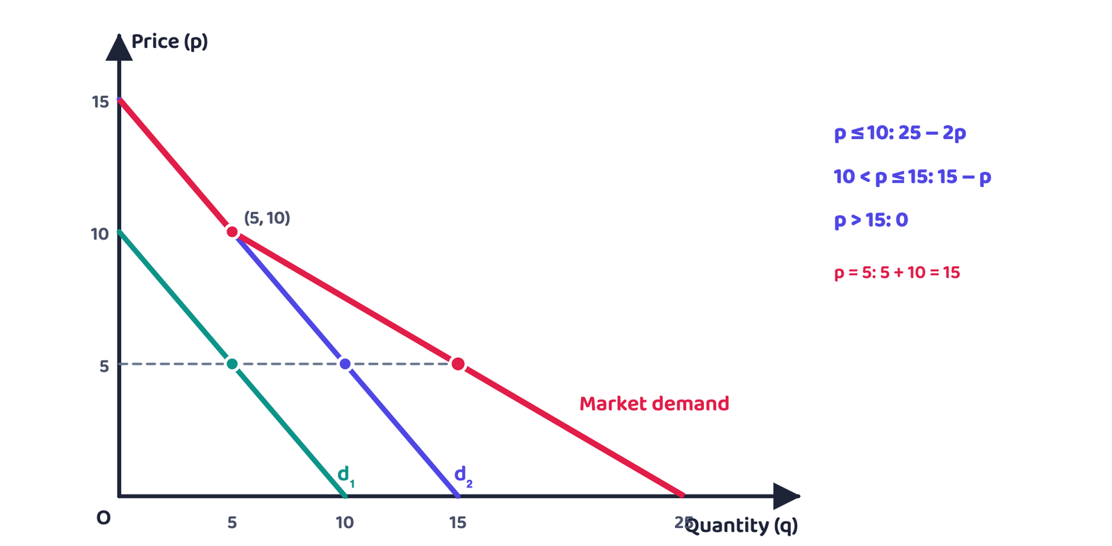
Two consumers: if at price p′ the demands are $q'_1$ and $q'_2$ , market demand is $q'_1 + q'_2$ ; the same addition is done at every price
Graphically the individual demand curves are added horizontally (quantities are added at each price, not prices); this method is horizontal summation

Book example: adding up two linear demand curves

$d_1(p) = 10 – p$ …(2.14), 0 at any price above 10; $d_2(p) = 15 – p$ …(2.15), 0 at any price above 15
p ≤ 10: both buy, market demand = (10 − p) + (15 − p) = 25 − 2p
10 < p ≤ 15: only consumer 2, market demand = 15 − p
p > 15: market demand = 0
Check: at p = 5, 5 + 10 = 15 = 25 − 2(5) ✓

Figure 14: Market demand: the horizontal sum of d₁ = 10 − p and d₂ = 15 − p; 25 − 2p for p ≤ 10, 15 − p between 10 and 15; a kink at price 10 — **Figure 14**: Market demand: the horizontal sum of d₁ = 10 − p and d₂ = 15 − p; 25 − 2p for p ≤ 10, 15 − p between 10 and 15; a kink at price 10

Common mistakes

Adding the two equations at every price is wrong; where a consumer’s demand would turn negative it is taken as 0 (so above 10 it is 15 − p, not 25 − 2p)
Adding prices (vertical summation) for a market curve is wrong; quantities are added

9 Price elasticity of demand

Demand moves opposite to price, but the impact is not always the same: some goods’ demand changes a lot even for small price changes, some hardly at all

Learn by heartDefinition 27

Price elasticity of demand is a measure of the responsiveness of the demand for a good to changes in its price: percentage change in demand for the good ÷ percentage change in its price.

Percentage method (2.16a, 2.16b)

e_D = \frac{\text{percentage change in demand}}{\text{percentage change in price}} = \frac{\frac{\Delta Q}{Q} \times 100}{\frac{\Delta P}{P} \times 100} = \frac{\Delta Q}{\Delta P} \times \frac{P}{Q}

ΔP = change in price, ΔQ = change in quantity; P and Q are the original values. Demand and price move in opposite directions, so

e_D

is a negative number; for simplicity its absolute value is used. Elasticity is a pure number (it has no unit).

Book’s Example 2.2

Q. At ₹5 per banana a consumer buys 15 bananas; when the price rises to ₹7 she buys 12. Find the price elasticity of demand.

Given

$P_1$ = 5, $P_2$ = 7; $Q_1$ = 15, $Q_2$ = 12

To find

$e_D$

% change in quantity $= \dfrac{Q_2 – Q_1}{Q_1} \times 100 = \dfrac{12 – 15}{15} \times 100 = -20$ (1)
% change in price $= \dfrac{P_2 – P_1}{P_1} \times 100 = \dfrac{7 – 5}{5} \times 100 = 40$ (1)
$e_D = \dfrac{20}{40} =$ 0.5 (absolute value) (1)
Meaning: price rose 40% and demand fell only 20%; demand for bananas is not very responsive to price, that is, inelastic

% change in quantity vs % change in price	$e_D$	Demand	Example (book)
Smaller	< 1	Inelastic	Essential goods
Larger	> 1	Elastic	Luxury goods
Equal	= 1	Unitary elastic	Rectangular hyperbola curve

The demand for a good may be elastic, unitary elastic or inelastic at different prices (next section).

Worked example 4: three kinds of percentage-method questions

Price ₹10 to ₹12, demand 100 to 80 units: % ΔQ = −20, % ΔP = +20; $e_D$ = 20/20 = 1 (unitary elastic)
Price ₹10 to ₹8, demand 100 to 150 units: % ΔQ = +50, % ΔP = −20; $e_D$ = 50/20 = 2.5 (elastic)
Elasticity given: $e_D$ = −1.5, price rises 20%, demand was 500 units; new demand? % ΔQ = −1.5 × 20 = −30; new demand = 500 × (1 − 0.30) = 350 units

Meaning: the higher the elasticity, the more demand changes for the same price change.

Common mistakes

Dividing by the new value when finding percentages is wrong; always divide by the original price and quantity (P, Q)
Inverting the formula ( $\Delta P/\Delta Q \times Q/P$ ) is wrong; the percentage change in quantity goes on top
Calling $e_D$ = −0.8 “elastic” is wrong; the absolute value 0.8 < 1, so it is inelastic

9.1 Elasticity along a linear demand curve

On the linear demand curve $q = a – bp$ , at every point $\dfrac{\Delta q}{\Delta p} = -b$ ; putting this in (2.16b) gives $e_D = -b\dfrac{p}{q}$ , and putting in the value of q:

Elasticity on a linear demand curve (2.17)

e_D = -\frac{bp}{a – bp}

At p = 0 elasticity is 0; at q = 0 (p = a/b) it is ∞; at p = a/2b (the midpoint) it is 1; at any price between 0 and a/2b it is less than 1; at any price above a/2b it is greater than 1.

Figure 15: Elasticity on the linear demand curve q = 10 − 3p: infinite at B, 1 at the midpoint M (p = 5/3), 1.5 at D (4, 2) = DA/DB, 0 at A — **Figure 15**: Elasticity on the linear demand curve q = 10 − 3p: infinite at B, 1 at the midpoint M (p = 5/3), 1.5 at D (4, 2) = DA/DB, 0 at A

Worked example 5: three points on a linear curve

Q. The demand curve is q = 100 − 5p. Find the elasticity at p = 4, 10 and 16.

Formula: $e_D = -\dfrac{bp}{a – bp}$ , here a = 100, b = 5 (½)
p = 4: q = 80, $e_D = -\dfrac{20}{80} =$ −0.25 (inelastic) (½)
p = 10: q = 50, $e_D = -\dfrac{50}{50} =$ −1 (unitary elastic); a/2b = 100/10 = 10, the midpoint (½)
p = 16: q = 20, $e_D = -\dfrac{80}{20} =$ −4 (elastic) (½)
Meaning: on one straight line the slope stays the same but elasticity rises as we move up; slope and elasticity are not the same thing

Geometric measure (Not in CBSE 2026-27 syllabus)

At any point on a straight-line demand curve, elasticity = the lower segment ÷ the upper segment at that point
At a point D on q = a − bp (price $p_0$ , quantity $q_0$ ; B on the vertical axis, A on the horizontal axis): similar triangles ECD, $Bp_0D$ and BOA give $e_D = \dfrac{q_0D}{p_0B} = \dfrac{DA}{DB}$
Elasticity is 0 where the curve meets the horizontal axis (A), ∞ where it meets the vertical axis (B), 1 at the midpoint; greater than 1 to the left of (above) the midpoint and less than 1 to the right of (below) it
In the figure above, at D (4, 2): DA/DB = (10 − 4)/(4 − 0) = 1.5, which the formula also gives: 3 × 2 ÷ (10 − 6) = 1.5

9.2 Constant elasticity demand curves

Vertical demand curve: whatever the price, demand stays at $\bar{q}$ ; $|e_D|$ = 0, perfectly inelastic
Horizontal demand curve: any quantity at the price $\bar{p}$ , zero demand at any other price; $e_D$ = ∞, perfectly elastic
Rectangular hyperbola (pq = constant): a percentage change in price always gives an equal percentage change in quantity; $|e_D|$ = 1 at every point, the unitary elastic demand curve

Figure 16: Constant elasticity demand curves: (a) vertical, e = 0; (b) horizontal, e = ∞; (c) rectangular hyperbola pq = 20, e = 1 at every point (equal rectangle areas) — **Figure 16**: Constant elasticity demand curves: (a) vertical, e = 0; (b) horizontal, e = ∞; (c) rectangular hyperbola pq = 20, e = 1 at every point (equal rectangle areas)

Rectangular hyperbola (the book’s box)

An equation xy = c (c a constant) gives a curve called a rectangular hyperbola, sloping downward in the x-y plane. For any two points on it, the rectangles under them have the same area (c). If a demand curve is pq = e, the consumer’s expenditure is always e, whichever point she consumes at.

9.3 Factors determining price elasticity of demand

Nature of the good

Necessities like food are essential for life, so their demand is inelastic; demand for luxuries is elastic

Close substitutes

Demand for food as a whole is inelastic, but for a particular variety of pulses it is elastic, because another variety is easily available. Without easily available close substitutes demand is inelastic

Time period (CBSE supplement)

Habits change over longer periods; the longer the period of response, the more elastic the demand

Share of income (CBSE supplement)

The higher the share of income spent on a good, the more elastic its demand; low priced goods have low elasticity

9.4 Elasticity and expenditure: the total expenditure method

Expenditure on a good = price × quantity demanded
Whether expenditure rises or falls when price changes depends on how responsive demand is to price

Row	Price (P)	Quantity (Q)	% ΔP	% ΔQ	Expenditure (P × Q)	Price elasticity of demand
1	↑	↓	+10	−8	↑	Inelastic
2	↑	↓	+10	−12	↓	Elastic
3	↑	↓	+10	−10	About unchanged	Unit elastic
4	↓	↑	−10	+15	↑	Elastic
5	↓	↑	−10	+7	↓	Inelastic
6	↓	↑	−10	+10	About unchanged	Unit elastic

Based on the book’s Table 2.5; each row’s expenditure and elasticity are recomputed from P × Q. In rows 3 and 6 expenditure is unchanged only approximately (1.1 × 0.9 = 0.99).

Rules of the total expenditure method

Elastic ( $e_D$ > 1): expenditure moves opposite to price (rows 2, 4). Inelastic ( $e_D$ < 1): expenditure moves in the same direction as price (rows 1, 5). Unit elastic ( $e_D$ = 1): expenditure unchanged (rows 3, 6).

Worked example 6: total expenditure method

Price ₹10 to ₹8, demand 100 to 150: expenditure ₹1,000 to ₹1,200; price fell, expenditure rose (opposite direction): elastic
Price ₹10 to ₹12, demand 60 to 50: expenditure ₹600 and ₹600; unchanged: unitary elastic
Price ₹4 to ₹5, demand 200 to 180: expenditure ₹800 to ₹900; price rose and expenditure also rose (same direction): inelastic. Check by the percentage method: % ΔQ = −10, % ΔP = +25, $e_D$ = 10/25 = 0.4 < 1 ✓

Change in expenditure and elasticity (the book’s box)

At price p demand is q, at p + Δp demand is q + Δq; the change in expenditure $= (p + \Delta p)(q + \Delta q) – pq = q\Delta p + p\Delta q + \Delta p\Delta q$
For small changes $\Delta p\Delta q$ is negligible, so $\Delta E \approx q\Delta p + p\Delta q = \Delta p\left[q\left(1 + \dfrac{\Delta q}{\Delta p}\dfrac{p}{q}\right)\right] = \Delta p[q(1 + e_D)]$
$e_D \lt -1$ : $\Delta E$ has the opposite sign to $\Delta p$ ; $e_D \gt -1$ : the same sign; $e_D = -1$ : $\Delta E = 0$

10 Key formulas and difference tables

Key formulas

MU_n = TU_n – TU_{n-1} \qquad TU_n = \sum MU

\text{One good: } MU = P \qquad \text{Two goods: } \frac{MU_x}{P_x} = \frac{MU_y}{P_y}

MRS = \left|\frac{\Delta Y}{\Delta X}\right| \qquad p_1x_1 + p_2x_2 = M \qquad \text{slope} = -\frac{p_1}{p_2}

\text{Equilibrium: } MRS = \frac{p_1}{p_2} \qquad e_D = \frac{\Delta Q}{\Delta P} \times \frac{P}{Q} \qquad e_D = -\frac{bp}{a – bp}

Basis	Normal good	Inferior good
Demand when income rises	Rises	Falls
Demand curve when income rises	Rightward	Leftward
Examples	Most goods, better quality cereals	Coarse cereals, low quality food

Basis	Perfectly elastic	Perfectly inelastic
$e_D$	∞	0
Demand curve	Horizontal	Vertical
Meaning	A small price change makes demand zero	Whatever the price, demand stays the same

All definitions in one place

Utilitywant-satisfying capacity of a commodity

Cardinal utility analysisutility can be measured in numbers

Total utilitytotal satisfaction from a given amount

Marginal utilitychange in TU from one additional unit

Law of diminishing marginal utilitywith other consumption constant, MU of each further unit falls

Demandquantity a consumer is willing to buy and able to afford at given prices and income

Consumer’s equilibriummaximum satisfaction for given income and prices

Ordinal utility analysisbundles are only ranked

Indifference curvecurve of bundles giving equal satisfaction

Marginal rate of substitutionmangoes given up for an extra banana, |ΔY/ΔX|

Law of diminishing MRSMRS falls as bananas increase

Perfect substitutesused in place of each other, exactly the same utility; IC a straight line

Monotonic preferencesmore of at least one good and no less of the other is preferred

Indifference mapa family of indifference curves

Budget constraint

p_1x_1 + p_2x_2 \le M

Budget setall bundles affordable with the income

Budget linebundles costing exactly M

Rational consumeralways chooses the most preferred available bundle

Demand functionX = f(P)

Demand scheduletable of quantities demanded at different prices

Law of demandother things equal, negative relation between price and demand

Normal gooddemand moves with income

Inferior gooddemand moves opposite to income

Complementsused together; demand moves opposite to the complement’s price

Substitutesused in place of each other; demand moves with the substitute’s price

Market demandtotal demand of all consumers at a price

Price elasticity of demand% change in demand ÷ % change in price

Quick recap: read this the night before

MU = TUn − TUn−1; TU is maximum when MU = 0; then MU is negative
One good: MU = P; two goods: MUx/Px = MUy/Py and MU falling
IC: equal satisfaction; slopes down, convex, a higher curve gives more satisfaction, curves never intersect
MRS = |ΔY/ΔX|, diminishing (Table 2.2: 3, 2, 1); constant for perfect substitutes, IC a straight line
Budget line $p_1x_1 + p_2x_2 = M$ ; intercepts M/p1, M/p2; slope −p1/p2
Income changes: parallel shift; p1 changes: pivot about the vertical intercept
Optimum: tangency, MRS = p1/p2, IC convex
Price falls: substitution effect + income effect, demand rises; Giffen good the exception
Own price changes: movement along; income, related prices, tastes change: shift
Market demand: horizontal sum; d1 = 10 − p, d2 = 15 − p ⇒ 25 − 2p (p ≤ 10)
eD = (ΔQ/ΔP)(P/Q); linear curve: −bp/(a − bp), 1 at the midpoint
Elastic: expenditure opposite to price; inelastic: same direction; unitary: unchanged

Check yourself before the exam

Can I work out MU from a TU table and draw the TU-MU diagram?
Can I write the MUx/Px = MUy/Py condition and the “a rupee from Y to X” argument?
Can I find MRS from Table 2.2 and draw a convex indifference curve?
Can I prove that two indifference curves cannot intersect?
Can I write the budget line, its intercepts and slope from any income and prices?
Can I draw the tangency equilibrium (E, x1*, x2*)?
Can I explain movement vs shift with diagrams?
Can I find elasticity by the percentage method, the linear-curve formula and the total expenditure method?

More for this chapter

Important Questions MCQ / Objective NCERT Solutions Short Notes