
Covers T.R. Jain & V.K. Ohri (2026-27) ch 4. Based on NCERT Statistics for Economics (Reprint 2026-27), Chapter 3. For CBSE, UP, Bihar, Rajasthan and MP Boards.
- What classification is and why raw data must be classified
- The four types of classification: chronological, spatial, qualitative and quantitative
- The difference between continuous and discrete variables
- How to make a frequency distribution: class limits, class interval, class mark, tally marks
- Inclusive and exclusive methods, adjustment of class intervals, unequal classes
- Frequency array and bivariate frequency distribution
1 What Is Classification?
Once data have been collected (from primary or secondary sources), the next job is to bring order in them, so that further statistical analysis can be done easily.
- The kabadiwallah buys old newspapers, broken household items, empty glass bottles and plastics from you and sells them to those who recycle them
- He ties old newspapers together with a rope, collects empty bottles in a sack, and sorts metal articles into “iron”, “copper”, “aluminium”, “brass”
- So his junk falls into classes: “newspapers”, “plastics”, “glass”, “metals”; under “glass” go empty bottles, broken mirrors and windowpanes
- Now any item a buyer asks for is found at once
In the same way, if you keep your schoolbooks subject-wise, a history book is searched for only in the group “History”, not in the whole pile. Put a book of another subject in that group and the whole purpose of grouping is lost.
Classification is arranging or organising things into groups or classes based on some criteria.
- Classification saves time and effort
- It is not done in an arbitrary manner: the kabadiwallah groups his junk according to the markets for reused goods
- Each group must hold things of one kind only
Sorting letters at a post office is also classification. The pin-code on a letter tells the postal area it goes to, so letters are sorted area-wise.
2 Raw Data
Raw data or unclassified data are data as collected, not yet arranged in any order or class.
The book gives two examples: Table 3.1 (marks in mathematics of 100 students in an examination) and Table 3.2 (monthly household expenditure on food of 50 households, in rupees). Table 3.1 is below; every example in the chapter is built from it.
| Table 3.1: Marks in Mathematics Obtained by 100 Students in an Examination | |||||||||
|---|---|---|---|---|---|---|---|---|---|
| 47 | 45 | 10 | 60 | 51 | 56 | 66 | 100 | 49 | 40 |
| 60 | 59 | 56 | 55 | 62 | 48 | 59 | 55 | 51 | 41 |
| 42 | 69 | 64 | 66 | 50 | 59 | 57 | 65 | 62 | 50 |
| 64 | 30 | 37 | 75 | 17 | 56 | 20 | 14 | 55 | 90 |
| 62 | 51 | 55 | 14 | 25 | 34 | 90 | 49 | 56 | 54 |
| 70 | 47 | 49 | 82 | 40 | 82 | 60 | 85 | 65 | 66 |
| 49 | 44 | 64 | 69 | 70 | 48 | 12 | 28 | 55 | 65 |
| 49 | 40 | 25 | 41 | 71 | 80 | 0 | 56 | 14 | 22 |
| 66 | 53 | 46 | 70 | 43 | 61 | 59 | 12 | 30 | 35 |
| 45 | 44 | 57 | 76 | 82 | 39 | 32 | 14 | 90 | 25 |
2.1 Problems with raw data
- They are highly disorganised, often very large and cumbersome to handle
- They do not yield to statistical methods easily, so drawing meaningful conclusions is a tedious task
- To find the highest mark in Table 3.1 you must first arrange all 100 marks in ascending or descending order; with 1,000 students it is more tedious still
- Finding the average monthly expenditure of the 50 households in Table 3.2 is difficult; with 5,000 households the difficulty goes up manifold
- Census: the Government of India conducts a census of population every ten years. About 20 crore persons were contacted in Census 2001. Such large, fragmented raw data seem almost impossible to draw conclusions from, but classified by gender, education, marital status and occupation, the structure and nature of India’s population are easily understood
Raw data consist of observations on variables (Table 3.1 holds 100 observations on the variable “marks in mathematics”). How we classify data depends on the purpose: a mathematics teacher who wants to know how her students have done and how many have not passed would probably construct a frequency distribution (Section 5).
3 Classification of Data: Four Types
Books can be classified by subject, by author in alphabetical order, or by year of publication; the choice depends on the requirement. Data too are classified in various ways depending on the purpose.
3.1 Chronological classification
Chronological classification: data classified in ascending or descending order with reference to time, such as years, quarters, months, weeks.
Time series: a series of values of a variable for different years (points of time). In Example 1 the variable “population” is a time series.
| Year | 1951 | 1961 | 1971 | 1981 | 1991 | 2001 | 2011 |
|---|---|---|---|---|---|---|---|
| Population (crores) | 35.7 | 43.8 | 54.6 | 68.4 | 81.8 | 102.7 | 121.0 |
Example 1: Population of India (in crores)
Minimum population: 1951 (35.7 crore); maximum: 2011 (121.0 crore).
Range = largest − smallest = 121.0 − 35.7 = 85.3 crore
3.2 Spatial classification
Spatial classification: data classified with reference to geographical locations such as countries, states, cities, districts.
| Country | Yield of wheat (kg/hectare) |
|---|---|
| Canada | 3594 |
| China | 5055 |
| France | 7254 |
| Germany | 7998 |
| India | 3154 |
| Pakistan | 2787 |
Example 2: Yield of wheat for different countries (2013). Source: Indian Agricultural Statistics at a Glance, 2015
Slightly more than India: Canada (3594). Difference = 3594 − 3154 = 440
In percentage = (440 ÷ 3154) × 100 = 13.95% more
Ascending order: Pakistan (2787) < India (3154) < Canada (3594) < China (5055) < France (7254) < Germany (7998); descending is the reverse.
Range = 7998 − 2787 = 5211
3.3 Qualitative classification
Attributes (qualities): characteristics that cannot be expressed quantitatively, i.e. cannot be measured; e.g. nationality, literacy, religion, gender, marital status.
Qualitative classification: classification of data on attributes on the basis of the presence or absence of a qualitative characteristic.
- First stage: presence or absence of an attribute, i.e. male or not male (female)
- Second stage: each class is further divided on another attribute (married or unmarried)
- The book’s activity: grouping objects around you as living or non-living is not quantitative; it is qualitative classification, since “being living” cannot be measured
3.4 Quantitative classification
Quantitative classification: grouping into classes the data of quantitative (measurable) characteristics such as height, weight, age, income, marks of students.
Example 4 (in Section 5) is the quantitative classification of the marks of 100 students from Table 3.1.
Calling a table of “literate/illiterate” or “male/female” counts a quantitative classification. Having numbers in it does not make it quantitative; its basis is an attribute, so it is qualitative. Likewise a state-wise table is spatial and a year-wise table is chronological.
4 Variables: Continuous and Discrete
Variable: a quantity whose values vary, such as the production of foodgrains year to year, students’ marks, income or household size. Variables are written as X, Y, Z, and each value of a variable is an observation (Chapter 2).
This simple definition does not tell how a variable varies. On that basis variables are of two types: (i) continuous and (ii) discrete.
Continuous variable: a variable that can take any numerical value: integral values (1, 2, 3), fractional values (1/2, 2/3, 3/4) and values that are not exact fractions (, , ).
Discrete variable: a variable that can take only certain values; its value changes only by finite “jumps” and it takes no intermediate value between two values.
Height (a continuous variable): growing from 90 cm to 150 cm it takes every value in between, whole numbers and fractions.
Continuous variable
- Can take every value in between
- Values can be broken down into infinite gradations
- Height: 90 cm, 100 cm, 102.34 cm, 149.99 cm
- Weight, time, distance
Discrete variable
- Only certain values; changes by “jumps”
- No value between two adjacent values
- Number of students in a class: 25 or 26, never 25.5 (“half a student” is absurd)
- Size of household, number of cars on road
“A discrete variable can never be a fraction” is wrong. Suppose X takes the values 1/8, 1/16, 1/32, 1/64 … X takes fractional values, yet it is discrete, because it jumps from 1/8 to 1/16 and takes no value between these two adjacent fractions. The test is “can it take a value in between?”, not “is it a whole number?”.
| Variable (book’s activity) | Type | Reason |
|---|---|---|
| Area, volume, temperature | Continuous | Measured; any value in between is possible |
| Number appearing on a dice | Discrete | Only 1, 2, 3, 4, 5, 6 |
| Crop yield, rainfall | Continuous | Any value in kilograms or millimetres |
| Population, number of cars on road | Discrete | Counted, only whole numbers |
| Age | Continuous | A measure of time; 15 years 4 months 10 days is possible |
Count it: discrete. Measure it: continuous.
What is counted (students, cars, family members) is discrete; what is measured (height, weight, time, rainfall) is continuous.
5 What Is a Frequency Distribution?
Frequency distribution: a comprehensive way to classify raw data of a quantitative variable, showing how the different values of the variable are distributed in different classes along with their corresponding class frequencies.
| Marks | 0-10 | 10-20 | 20-30 | 30-40 | 40-50 | 50-60 | 60-70 | 70-80 | 80-90 | 90-100 | Total |
|---|---|---|---|---|---|---|---|---|---|---|---|
| Frequency | 1 | 8 | 6 | 7 | 21 | 23 | 19 | 6 | 5 | 4 | 100 |
Example 4: Frequency distribution of marks in mathematics of 100 students (from Table 3.1)
5.1 Terms of a frequency distribution
Class frequency: the number of values in a particular class. The class 30-40 has 7 values from Table 3.1: 30, 37, 34, 30, 35, 39, 32; so its frequency is 7.
Class limits: the two ends of a class. The lowest value is the lower class limit and the highest value the upper class limit. For the class 60-70 they are 60 and 70.
Class interval or class width: the difference between the upper class limit and the lower class limit. For 60-70 it is 70 − 60 = 10.
Class mid-point or class mark: the middle value of a class, halfway between its lower and upper class limits. It is used to represent the class.
| Class | Frequency | Lower class limit | Upper class limit | Class mark |
|---|---|---|---|---|
| 0-10 | 1 | 0 | 10 | 5 |
| 10-20 | 8 | 10 | 20 | 15 |
| 20-30 | 6 | 20 | 30 | 25 |
| 30-40 | 7 | 30 | 40 | 35 |
| 40-50 | 21 | 40 | 50 | 45 |
| 50-60 | 23 | 50 | 60 | 55 |
| 60-70 | 19 | 60 | 70 | 65 |
| 70-80 | 6 | 70 | 80 | 75 |
| 80-90 | 5 | 80 | 90 | 85 |
| 90-100 | 4 | 90 | 100 | 95 |
Table 3.3: The lower class limits, the upper class limits and the class mark
Frequency curve: a graphic representation of a frequency distribution, with class marks on the X-axis and frequency on the Y-axis.

5.2 Relative frequency
Relative frequency: the frequency of a class expressed as a proportion or percentage of the total frequency. Relative frequency = class frequency ÷ total frequency.
The total frequency is 100, so each frequency is also the percentage: 0-10 = 1/100 = 0.01 = 1%; 10-20 = 0.08 = 8%; … 50-60 = 0.23 = 23%.
Maximum concentration: class 50-60, 23% of observations. Minimum concentration: class 0-10, 1%.
6 How to Prepare a Frequency Distribution: Five Questions
6.1 Equal or unequal class intervals?
Unequal sized class intervals are used in two situations:
- When the range is very high, as with income: income per day may range from nearly zero to many hundred crores of rupees. Equal classes do not suit this because (i) with moderate, equal intervals there would be a large number of classes; (ii) with large intervals, information on very small or very high levels of income would be suppressed
- When a large number of values are concentrated in a small part of the range: equal class intervals would lead to lack of information on many values
In all other cases equal sized class intervals are used.
6.2 How many classes, and what size?
Range: the difference between the largest and the smallest values of a variable. Range = largest value − smallest value.
- The number of classes and the size of each class are interlinked: one cannot be decided without the other
- Example 4: range = 100 − 0 = 100 and 10 classes were chosen, so the class interval is automatically 100 ÷ 10 = 10
- Equal intervals were chosen here; unequal ones could have been chosen too, giving classes of unequal width
6.3 How to determine class limits?
- Class limits should be definite and clearly stated
- Generally, open-ended classes such as “70 and over” or “less than 10” are not desirable, because one limit is left open
- Limits should be set so that the frequencies of each class tend to concentrate in the middle of the class interval
6.4 Inclusive and exclusive class intervals
Inclusive class intervals: values equal to both the lower and the upper limits of a class are included in the frequency of that same class.
Exclusive class intervals: an item equal to either the upper or the lower class limit is excluded from the frequency of that class.
Inclusive form (marks 0 to 100)
- 0-10, 11-20, 21-30, …, 91-100
- A mark of 10 goes to 0-10, 11 to 11-20
- There is a “gap” between the upper limit of one class and the lower limit of the next
Exclusive form (marks 0 to 100)
- 0-10, 10-20, 20-30, …, 90-100
- Upper limit of one class = lower limit of the next
- We must decide in advance where a value equal to a limit goes
For a value equal to a class limit (10, 30 etc.) in the exclusive method, there are two choices:
- Put 10, 30 into “0 to 10” and “20 to 30”: the case of lower limit excluded
- Put 10, 30 into “10 to 20” and “30 to 40”: the case of upper limit excluded. The book’s Example 4 follows this (a mark of 40 is counted in 40-50)
- The book: for discrete variables, both exclusive and inclusive class intervals can be used. Whole-number marks (no fractional marks allowed) are a discrete variable
- The book: “In the case of continuous variables, inclusive class intervals are used very often.” Classes of height (cm) or weight (kg) are written as 30 Kg – 39.999… Kg, 40 Kg – 49.999… Kg, meaning “30 Kg and above and under 40 Kg“, “40 Kg and above and under 50 Kg” and so on. Note: in meaning these are exclusive classes; continuous classes written in the inclusive form (such as 800-899) are made continuous by the adjustment below
6.5 Adjustment in class interval
In Table 3.4, “income” is a continuous variable, but its inclusive classes leave a “gap” (discontinuity): between the upper limit of the first class, 899, and the lower limit of the second, 900, there is a gap of 1. Continuity is restored by an adjustment in the class interval.
| Table 3.4: Income (Rs) | Table 3.5: Adjusted income (Rs) | Number of employees | Class mark |
|---|---|---|---|
| 800-899 | 799.5-899.5 | 50 | 849.5 |
| 900-999 | 899.5-999.5 | 100 | 949.5 |
| 1000-1099 | 999.5-1099.5 | 200 | 1049.5 |
| 1100-1199 | 1099.5-1199.5 | 150 | 1149.5 |
| 1200-1299 | 1199.5-1299.5 | 40 | 1249.5 |
| 1300-1399 | 1299.5-1399.5 | 10 | 1349.5 |
| Total | 550 |
Frequency distribution of incomes of 550 employees of a company, before and after adjustment
Adding 0.5 only to the upper limits, or subtracting it only from the lower limits. Adjustment changes both limits; only then does each upper limit equal the next lower limit (899.5 = 899.5). And it is not always 0.5: it is half the gap, so a gap of 0.1 gives 0.05.
7 Finding Class Frequency by Tally Marking
In simple terms, the frequency of an observation means how many times it occurs in the raw data. In Table 3.1 the value 40 occurs thrice, 0 and 10 once each, and 49 five times. When data are grouped into classes, the class frequency is the number of values in a class, counted by tally marks.
Tally marks: a tally (/) put against a class for each observation in it. Four tallies are put as //// and the fifth is placed across them, so tallies are counted in groups of five. The frequency of a class = the number of tallies against it.
- 57 marks: a tally against 50-60
- 71 marks: against 70-80
- 40 marks: against 40-50 (upper limit excluded)
- 16 tallies = three crossed groups of five + 1:
|||||||||||||
| Class | Observations (from Table 3.1) | Tally | Frequency | Class mark |
|---|---|---|---|---|
| 0-10 | 0 | | | 1 | 5 |
| 10-20 | 10, 14, 17, 12, 14, 12, 14, 14 | 8 | 15 | |
| 20-30 | 25, 25, 20, 22, 25, 28 | 6 | 25 | |
| 30-40 | 30, 37, 34, 39, 32, 30, 35 | 7 | 35 | |
| 40-50 | 47, 42, 49, 49, 45, 45, 47, 44, 40, 44, 49, 46, 41, 40, 43, 48, 48, 49, 49, 40, 41 | 21 | 45 | |
| 50-60 | 59, 51, 53, 56, 55, 57, 55, 51, 50, 56, 59, 56, 59, 57, 59, 55, 56, 51, 55, 56, 55, 50, 54 | 23 | 55 | |
| 60-70 | 60, 64, 62, 66, 69, 64, 64, 60, 66, 69, 62, 61, 66, 60, 65, 62, 65, 66, 65 | 19 | 65 | |
| 70-80 | 70, 75, 70, 76, 70, 71 | 6 | 75 | |
| 80-90 | 82, 82, 82, 80, 85 | 5 | 85 | |
| 90-100 | 90, 100, 90, 90 | |||| | 4 | 95 |
| Total | 100 | |||
Table 3.6: Tally marking of marks of 100 students in mathematics (the last class 90-100 also holds the mark 100)
The book asks why 40, which occurs in the raw data, is not counted in the class 30-40. Answer: the classes 30-40, 40-50 are exclusive with the upper limit excluded, so 40 goes to 40-50. All 7 values in 30-40 are below 40.
Q. Daily wages (₹) of 20 workers: 212, 245, 230, 268, 251, 239, 222, 275, 260, 248, 233, 255, 241, 219, 266, 227, 250, 236, 244, 258. Make an exclusive frequency distribution with a class interval of 10.
Step 1 (range): largest = 275, smallest = 212; range = 275 − 212 = 63
Step 2 (number of classes): 63 ÷ 10 = 6.3, i.e. 7 classes, starting at 210: 210-220, 220-230, …, 270-280
Step 3 (tallies): each value against its class; 230, 250 and 260 go to the class that begins with them (upper limit excluded)
Step 4 (count and check): total of frequencies = number of observations = 20
| Wage (₹) | 210-220 | 220-230 | 230-240 | 240-250 | 250-260 | 260-270 | 270-280 | Total |
|---|---|---|---|---|---|---|---|---|
| Tally | || | || | |||| | |||| | |||| | ||| | | | |
| Frequency | 2 | 2 | 4 | 4 | 4 | 3 | 1 | 20 |
| Class mark | 215 | 225 | 235 | 245 | 255 | 265 | 275 |
Interpretation: 12 of the 20 workers (60%) earn between ₹230 and ₹260; wages are concentrated in this middle range.
(1) Not checking that the frequencies add up to the number of observations: that total is the check on your counting. (2) Missing the largest value: the last upper limit must exceed the largest value (or equal it, in the inclusive form). (3) Counting a value at a limit twice in exclusive classes.
8 Loss of Information
Loss of information: once data are grouped into a frequency distribution, the actual values of the observations in a class are lost and further statistical calculations are based only on the class mark; this inherent shortcoming of classification is the loss of information.
The class 20-30 contains 6 observations: 25, 25, 20, 22, 25 and 28. The frequency distribution gives only the frequency, 6, not the actual values. All values in this class are assumed equal to the class mark, 25. The same is true for every class.
Still, classification makes raw data concise and comprehensible; being able to make more sense of the data more than makes up for this loss.
9 Frequency Distribution with Unequal Classes
- In Example 4 most observations are concentrated in 40-50, 50-60 and 60-70; the other seven classes are sparsely populated, and the book notes that observations in those sparse classes deviate more from their class marks
- If classes are formed so that class marks coincide, as far as possible, with the value around which the observations in a class tend to concentrate, unequal class intervals are more appropriate
- In Table 3.7, 40-50 is split into 40-45 and 45-50, 50-60 into 50-55 and 55-60, and 60-70 into 60-65 and 65-70 (interval 5); the other classes keep the interval 10
- The observations deviate more from the old class marks than from the new ones, so the new class marks are more representative of the data
| Class | 0-10 | 10-20 | 20-30 | 30-40 | 40-45 | 45-50 | 50-55 | 55-60 | 60-65 | 65-70 | 70-80 | 80-90 | 90-100 |
|---|---|---|---|---|---|---|---|---|---|---|---|---|---|
| Frequency | 1 | 8 | 6 | 7 | 9 | 12 | 7 | 16 | 10 | 9 | 6 | 5 | 4 |
| Class mark | 5 | 15 | 25 | 35 | 42.5 | 47.5 | 52.5 | 57.5 | 62.5 | 67.5 | 75 | 85 | 95 |
Table 3.7: Frequency distribution of unequal classes (total 100)

Fig 3.2 has six points in the middle range (40-70) where Fig 3.1 has three, so it can show that marks are denser in 45-50 and 55-60. The curve is more uneven and closer to the actual spread of the data. Outside this range (0-40, 70-100) the two curves are the same. Note: the frequencies of the narrower classes (interval 5) are naturally smaller, since each old class is split into two.
10 Frequency Array
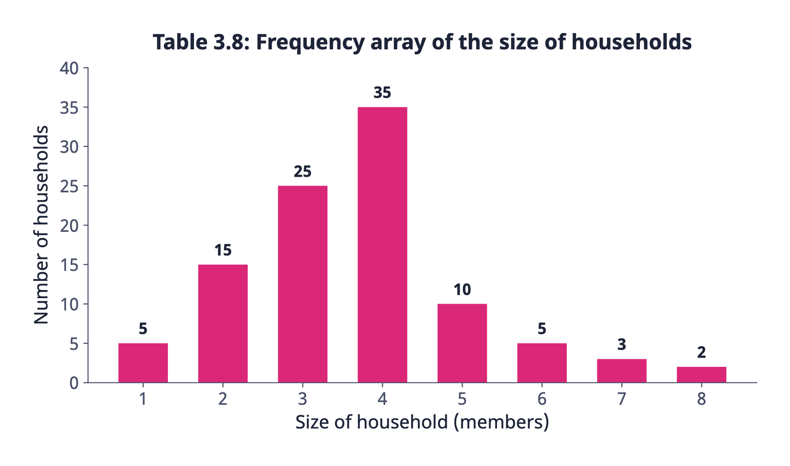
Frequency array: the classification of data of a discrete variable, in which the frequency is written against each value of the variable (no classes are formed).
| Size of household | 1 | 2 | 3 | 4 | 5 | 6 | 7 | 8 | Total |
|---|---|---|---|---|---|---|---|---|---|
| Number of households | 5 | 15 | 25 | 35 | 10 | 5 | 3 | 2 | 100 |
Table 3.8: Frequency array of the size of households. “Size of the household” is a discrete variable taking only integral values.
Frequency array
- Discrete variable
- Frequency of each separate value
- No class limits
- Example: size of household
Frequency distribution (with classes)
- Mainly a continuous variable (or a discrete one with very many values)
- Frequency of classes (intervals)
- Class limits, class marks
- Example: marks, income
11 Bivariate Frequency Distribution
When we take a sample from a population, we often collect more than one type of information from each element. Suppose we take a sample of 20 companies from the list of companies based in a city and collect information on sales and expenditure on advertisements from each. This is bivariate sample data.
Bivariate frequency distribution: the frequency distribution of two variables. (The distribution of a single variable is a univariate frequency distribution.)
| Advertisement (Rs thousand) ↓ / Sales (Rs lakh) → | 115-125 | 125-135 | 135-145 | 145-155 | 155-165 | 165-175 | Total |
|---|---|---|---|---|---|---|---|
| 62-64 | 2 | 1 | 3 | ||||
| 64-66 | 1 | 3 | 4 | ||||
| 66-68 | 1 | 1 | 2 | 1 | 5 | ||
| 68-70 | 2 | 2 | 4 | ||||
| 70-72 | 1 | 1 | 1 | 1 | 4 | ||
| Total | 4 | 5 | 6 | 3 | 1 | 1 | 20 |
Table 3.9: Bivariate frequency distribution of sales (in lakh Rs) and advertisement expenditure (in thousand Rs) of 20 firms
- Values of sales are classed in different columns and values of advertisement expenditure in different rows
- Each cell shows the frequency of the corresponding row and column values: 3 firms have sales between Rs 135 and Rs 145 lakh and advertisement expenditure between Rs 64 and Rs 66 thousand
- The last column (totals) gives the univariate distribution of advertisement expenditure alone, and the last row that of sales alone; both add up to 20
- The bivariate distribution is used later in the chapter on correlation
Univariate frequency distribution
- One variable
- Classes in one column, frequencies in another
- Example: marks of 100 students
Bivariate frequency distribution
- Two variables together
- One variable in rows, the other in columns; frequencies in cells
- Example: sales and advertisement expenditure of 20 firms
12 Key Formulas and Difference Tables
| Basis | Raw data | Classified data |
|---|---|---|
| Arrangement | Not in any order | Ordered into classes |
| Size | Large, hard to handle | Concise and comprehensible |
| Comparison and inference | Difficult, tedious | Easy |
| Information | Every actual value available | Actual values lost (loss of information) |
| Basis | Inclusive method | Exclusive method |
|---|---|---|
| Values at limits | Both limits included in the class | One limit excluded (the upper, in Example 4) |
| Form of classes | 0-10, 11-20, 21-30 | 0-10, 10-20, 20-30 |
| Continuity | Gaps between classes; a continuous variable needs adjustment | Upper limit = next lower limit, continuous |
| Basis | Equal class intervals | Unequal class intervals |
|---|---|---|
| When | The normal case | Very large range (income), or values concentrated in a small part |
| Example | Example 4 (all classes of 10) | Table 3.7 (some classes of 5) |
| Basis | Qualitative classification | Quantitative classification |
|---|---|---|
| Basis | Attributes that cannot be measured | Measurable characteristics |
| How | Presence or absence of an attribute | Classes (intervals) of values |
| Examples | Gender, religion, literacy, marital status | Height, weight, age, income, marks |
| Basis | Chronological classification | Spatial classification |
|---|---|---|
| Basis | Time (years, quarters, months) | Place (countries, states, districts) |
| Example | Population of India 1951-2011 | Yield of wheat by country, 2013 |
- Classification brings order to raw data
- Four types: chronological (time), spatial (place), qualitative (attribute), quantitative (measurement)
- Continuous: every value in between; discrete: changes by jumps (1/8, 1/16 is also discrete)
- Frequency distribution: values of a variable in classes, with class frequencies
- Class mark = (upper + lower) ÷ 2; class interval = upper − lower; range = largest − smallest
- Usually six to fifteen classes; open-ended classes are not desirable
- Exclusive method: the upper or the lower limit is excluded (Example 4 excludes the upper); inclusive method: both limits included
- Adjustment: half the gap subtracted from lower limits and added to upper limits (800-899 → 799.5-899.5)
- Tallies in groups of five; frequencies add up to the total observations
- Further calculations use only class marks: loss of information
- Class marks should lie near the value around which observations concentrate: hence sometimes unequal classes
- A discrete variable is classified as a frequency array; two variables give a bivariate distribution (Table 3.9, 20 firms)
- Can I tell from a table whether the classification is chronological, spatial, qualitative or quantitative?
- Can I show why a variable taking 1/8, 1/16 is discrete?
- Can I find the range, number of classes, tallies and frequency distribution from raw data, and check the total?
- Can I adjust inclusive classes and find class marks?
- Can I explain loss of information with the class 20-30 example?
- Can I write the meaning of any cell of a bivariate table?