
Covers T.R. Jain & V.K. Ohri (2026-27) ch 11. Based on NCERT Statistics for Economics, Chapter 6 (Reprint 2026-27) and the CBSE curriculum 2026-27 (Part A, Unit 3).
- State what correlation means and tell correlation apart from cause and effect
- Recognise positive, negative, linear and non-linear relations and draw scatter diagrams
- Calculate Karl Pearson’s coefficient of correlation (r) three ways: deviation method, direct method and step deviation method
- Write the properties of r and interpret its values (+1, −1, 0, 0.9, 0.1)
- Calculate Spearman’s rank correlation in all three cases: ranks given, ranks not given, and repeated ranks (with the correction factor)
1 Meaning of Correlation
- As the summer heat rises, hill stations are crowded with more visitors and ice-cream sales become more brisk
- So temperature is related to the number of visitors and the sale of ice-creams
- As the supply of tomatoes in the local mandi increases, its price drops: when the local harvest reaches the market, the price falls from Rs 40 per kg to Rs 4 per kg or even less
- So supply is related to price
- Correlation analysis is a means of examining such relationships systematically
Correlation studies and measures the direction and intensity of relationship among variables. Correlation measures covariation, not causation.
Correlation analysis answers four questions:
Any relationship?
Is there any relationship between two variables?
One changes, the other?
If the value of one variable changes, does the value of the other also change?
Direction
Do both the variables move in the same direction?
Intensity
How strong is the relationship?
2 Types of Relationship: Cause, Coincidence and a Third Variable
When two variables seem to move together, there can be three quite different reasons:
Cause and effect
The relation between quantity demanded and price is an integral part of the theory of demand (Class XII). Low agricultural productivity is related to low rainfall.
Simple coincidence
Arrival of migratory birds in a sanctuary and the birth rates in the locality; size of shoes and money in your pocket. Even if a relationship exists, it is difficult to explain.
A third variable
Brisk sale of ice-creams may be related to more deaths due to drowning, but the victims did not drown because they ate ice-cream. A third variable, temperature, is behind both.
- Rising temperature leads to brisk sale of ice-creams
- The same heat makes a large number of people go to swimming pools to beat the heat
- This might have raised the number of deaths by drowning
- So temperature is behind the high correlation between ice-cream sales and deaths due to drowning
Correlation measures covariation, not causation. Correlation should never be interpreted as implying cause and effect relation.
The book
| Basis | Correlation | Causation |
|---|---|---|
| What it says | In which direction and how strongly two variables change together | A change in one variable is the reason for the change in the other |
| Measure | A number r (−1 to +1) or a scatter diagram | No statistical measure; decided by theory and reasoning |
| Example | Ice-cream sales and deaths by drowning (high correlation) | Temperature ↑ ⇒ ice-cream sales ↑ |
| Link | Correlation can exist without causation | A causal relation that is not linear can still give r = 0 (as with y = x²) |
3 Types of Correlation
For simplicity the book assumes that the correlation, if it exists, is linear, i.e. the relative movement of the two variables can be represented by drawing a straight line on graph paper.
Positive correlation: the variables move together in the same direction; when one rises the other rises, and when one falls the other falls.
Negative correlation: the variables move in opposite directions; when one rises the other falls.
Positive correlation
- Both variables in the same direction
- Income rises, consumption rises; income falls, consumption falls
- Sale of ice-cream and temperature
- r positive (0 to +1)
Negative correlation
- Variables in opposite directions
- Price of apples falls, its demand increases; price rises, demand decreases
- More time spent studying, lower chances of failing
- r negative (0 to −1)
Linear relation: a relationship is said to be linear if it can be represented by a straight line. A relation that shows up as a curve rather than a straight line is a non-linear relation.
4 Techniques for Measuring Correlation
- Spearman’s coefficient measures the linear association between ranks assigned to individual items according to their attributes
- Attributes are variables which cannot be numerically measured, such as intelligence of people, physical appearance and honesty
5 Scatter Diagram
A scatter diagram is a useful technique for visually examining the form of relationship without calculating any numerical value: the values of the two variables are plotted as points on a graph paper.
- The degree of closeness of the scatter points and their overall direction tell us about the relationship
- If all the points lie on a line, the correlation is perfect and is said to be in unity
- If the points are widely dispersed around the line, the correlation is low
- The correlation is linear if the points lie near a line or on a line

| Book figure | Where the points lie | Relation |
|---|---|---|
| 6.1 | Scattered around an upward rising line | Positive correlation: when X rises, Y also rises |
| 6.2 | Scattered around a downward sloping line | Negative correlation: when X rises, Y falls and vice versa |
| 6.3 | No upward rising or downward sloping line | No correlation |
| 6.4 | The points themselves on a rising line | Perfect positive correlation (r = +1) |
| 6.5 | The points themselves on a falling line | Perfect negative correlation (r = −1) |
| 6.6 | Around a rising curve | Positive non-linear relation |
| 6.7 | Around a falling curve | Negative non-linear relation |
For a scatter diagram question, draw a small sketch, label the axes X and Y, and write the name of the relation under it. Of the three measures, only the scatter diagram can show any type of relationship, linear or non-linear; it is not confined to linear relations.
Collect data on height, weight and marks scored by students in your class in any two subjects in class X. Draw scatter diagrams taking two variables at a time and see what type of relationship you find.
6 Karl Pearson’s Coefficient of Correlation
Karl Pearson’s coefficient of correlation (r) gives a precise numerical value of the degree of linear relationship between two variables X and Y. It is also known as the product moment correlation coefficient or the simple correlation coefficient.
- Karl Pearson’s coefficient should be used only when there is a linear relation between the variables (Figs 6.1, 6.2, 6.4, 6.5)
- For a non-linear relation (Figs 6.6, 6.7), calculating it can be misleading
- So it is advisable to first examine the scatter diagram before calculating r
6.1 Quantities needed for r
Let be N values of X and the corresponding values of Y.
- Standard deviations are always positive
- So the sign of the covariance determines the sign of r
- If the covariance is zero, r is always zero
6.2 The four formulas for r
…(1)
…(2)
…(3)
…(4)
| Formula | Easiest when | Values needed |
|---|---|---|
| (1) covariance / SDs | σx, σy already known | Σxy, σx, σy, N |
| (2) deviation method | means are whole numbers | Σxy, Σx², Σy² |
| (3), (4) direct method | means are in decimals | ΣX, ΣY, ΣX², ΣY², ΣXY, N |
| Step deviation (section 10) | values are large | the same sums for U, V |
7 Properties of the Correlation Coefficient
No unit
r is a pure number; units of measurement are not part of r. r between height in feet and weight in kilograms could be, say, 0.7.
Negative r
An inverse relation: when the price of a commodity rises, its demand falls; when the rate of interest rises, the demand for funds falls, because funds have become costlier.
Positive r
Both move in the same direction: when the price of coffee, a substitute of tea, rises, the demand for tea rises; better irrigation goes with higher yield; higher temperature, brisker ice-cream sales.
Range −1 to +1
. If r is outside this range in any exercise, it indicates an error in calculation.
Unaffected by origin and scale
The magnitude of r is unaffected by change of origin and change of scale. The step deviation method rests on this.
r = 0
The two variables are uncorrelated: there is no linear relation between them. Other types of relation may still be there.
r = 1 or r = −1
The correlation is perfect and there is an exact linear relation.
High and low r
r close to +1 or −1 shows a strong linear relationship. r close to zero shows a weak linear relation, but there may be a non-linear relation.
What property 5 means: subtracting a number from every value (change of origin) or dividing every value by a number (change of scale) does not change r. The formula and a worked example are in section 10 (step deviation method).
“r = 0, so the two variables are independent” is wrong. r = 0 only means there is no linear relation. In Exercise 19, y = x² is an exact relation, yet r = 0.
7.1 Understand the data before interpreting r (book’s example)
- An epidemic spreads in some villages and the government sends a team of doctors to the affected villages
- The correlation between the number of deaths and the number of doctors sent was found to be positive
- Normally the healthcare provided by doctors is expected to reduce deaths, showing a negative correlation
- This happened due to other reasons: the data relate to a specific time period; many reported deaths could be terminal cases where the doctors could do little; the benefit of doctors becomes visible only after some time
- It is also possible that the reported deaths are not due to the epidemic: a tsunami suddenly hits the state and the death toll rises
- Lesson: statistical methods are no substitute for common sense
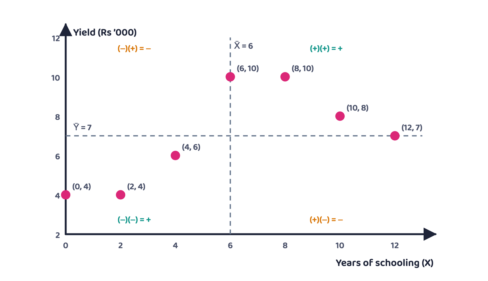
8 Worked Example 1: Farmers’ Schooling and Yield
Given
Years of schooling of farmers (X): 0, 2, 4, 6, 8, 10, 12; annual yield per acre in ’000 (Rs) (Y): 4, 4, 6, 10, 10, 8, 7; N = 7
To find
Karl Pearson’s coefficient of correlation r
Step 1: means. , . Both are whole numbers, so the deviation method is easiest.
Step 2: deviation table (book’s Table 6.1)
| X | x = X − X̄ | x² | Y | y = Y − Ȳ | y² | xy |
|---|---|---|---|---|---|---|
| 0 | −6 | 36 | 4 | −3 | 9 | 18 |
| 2 | −4 | 16 | 4 | −3 | 9 | 12 |
| 4 | −2 | 4 | 6 | −1 | 1 | 2 |
| 6 | 0 | 0 | 10 | 3 | 9 | 0 |
| 8 | 2 | 4 | 10 | 3 | 9 | 6 |
| 10 | 4 | 16 | 8 | 1 | 1 | 4 |
| 12 | 6 | 36 | 7 | 0 | 0 | 0 |
| ΣX = 42 | 0 | Σx² = 112 | ΣY = 49 | 0 | Σy² = 38 | Σxy = 42 |
Same by formula (1): , ;
Interpretation: years of education of farmers and annual yield per acre are positively correlated, and the value of r is also large. The more years farmers invest in education, the higher the yield per acre. It underlines the importance of farmers’ education.
By formula (3) (direct method): we need , , .
| X | Y | X² | Y² | XY |
|---|---|---|---|---|
| 0 | 4 | 0 | 16 | 0 |
| 2 | 4 | 4 | 16 | 8 |
| 4 | 6 | 16 | 36 | 24 |
| 6 | 10 | 36 | 100 | 60 |
| 8 | 10 | 64 | 100 | 80 |
| 10 | 8 | 100 | 64 | 80 |
| 12 | 7 | 144 | 49 | 84 |
| ΣX = 42 | ΣY = 49 | ΣX² = 364 | ΣY² = 381 | ΣXY = 336 |
(1) Σx and Σy always come to 0; if they do not, a mean or a deviation is wrong. (2) Forgetting that (−)(−) = + in the xy column. (3) Writing in the denominator instead of , which makes r far too small. (4) An r greater than 1 is impossible; recheck the working.
9 Interpreting Values of r
| Book’s example | r | Meaning |
|---|---|---|
| Marks in English and Statistics | 0.1 | Positive but weak: students with high marks in English may get relatively low marks in Statistics |
| Marks in English and Statistics | 0.9 | Strong positive: students with high marks in English will invariably get high marks in Statistics |
| Arrival of vegetables in the mandi and their price | −0.9 | Larger supply will be accompanied by a much lower price |
| Arrival of vegetables in the mandi and their price | −0.1 | Price falls, but not as low as when r is −0.9 |
| Arrival of vegetables in the mandi and their price | 0 | No fall in price even after large supplies; possible if a good transport network takes the extra supply to other markets |
The extent of the price fall depends on the absolute value of r (its value ignoring the sign).
10 Step Deviation Method
- When the values of the variables are large, the burden of calculation can be reduced by using a property of r
- The property: r is independent of change in origin and change in scale
- X and Y are transformed into U and V; the r of U and V is the same as
10.1 Worked Example 2: price index and money supply
Given
Price index (X): 120, 150, 190, 220, 230; money supply in Rs crores (Y): 1800, 2000, 2500, 2700, 3000; A = 100, h = 10, B = 1700, k = 100
To find
r by the step deviation method
| X | Y | U = (X − 100)/10 | V = (Y − 1700)/100 | U² | V² | UV |
|---|---|---|---|---|---|---|
| 120 | 1800 | 2 | 1 | 4 | 1 | 2 |
| 150 | 2000 | 5 | 3 | 25 | 9 | 15 |
| 190 | 2500 | 9 | 8 | 81 | 64 | 72 |
| 220 | 2700 | 12 | 10 | 144 | 100 | 120 |
| 230 | 3000 | 13 | 13 | 169 | 169 | 169 |
| ΣU = 41 | ΣV = 35 | ΣU² = 423 | ΣV² = 343 | ΣUV = 378 |
The strong positive correlation between price index and money supply is an important premise of monetary policy: when the money supply grows, the price index also rises. Applying formula (3) to the raw X and Y gives exactly the same 0.987.
(1) Subtracting A in some rows but forgetting to divide by h in others: every row must get the same transformation. (2) Mixing up Σ(U²) and (ΣU)²: 423 and 1681 are different numbers. (3) Taking h and k of opposite signs flips the sign of r.
Using data on India’s population and national income, calculate the correlation between them using the step deviation method. Both series have large values, which is exactly when this method helps.
10.2 Solving the book’s activity table
The book’s activity: calculate r between annual growth of national income at current price (X) and Gross Domestic Saving as percentage of GDP (Y) (Source: Economic Survey, (2004-05) Pg. 8, 9). The means 13.9 and 24.5 are decimals, so use the direct method (formula 3).
| Year | X | Y | X² | Y² | XY |
|---|---|---|---|---|---|
| 1992-93 | 14 | 24 | 196 | 576 | 336 |
| 1993-94 | 17 | 23 | 289 | 529 | 391 |
| 1994-95 | 18 | 26 | 324 | 676 | 468 |
| 1995-96 | 17 | 27 | 289 | 729 | 459 |
| 1996-97 | 16 | 25 | 256 | 625 | 400 |
| 1997-98 | 12 | 25 | 144 | 625 | 300 |
| 1998-99 | 16 | 23 | 256 | 529 | 368 |
| 1999-00 | 11 | 25 | 121 | 625 | 275 |
| 2000-01 | 8 | 24 | 64 | 576 | 192 |
| 2001-02 | 10 | 23 | 100 | 529 | 230 |
| Total | ΣX = 139 | ΣY = 245 | ΣX² = 2039 | ΣY² = 6019 | ΣXY = 3419 |
Interpretation: over these ten years, growth of national income and the saving rate show a positive but weak correlation.
11 Spearman’s Rank Correlation
Spearman’s rank correlation is the correlation coefficient in which individual values are replaced by their ranks. It measures the linear association between the ranks assigned to the units, not their values. It was developed by the British psychologist C.E. Spearman.
It is used in these situations:
No measuring tools
In a remote village with neither measuring rods nor weighing machines, height and weight cannot be measured, but students can be ranked by them.
Qualitative variables
Fairness, honesty or beauty cannot be measured like income or weight; at most they can be ranked. If at least one variable is of this type, use Spearman.
Clear direction, non-linear
Where the direction of the relation is clear but it is non-linear, as in Figs 6.6 and 6.7.
Extreme values
Spearman’s coefficient is not affected by extreme values. In this respect it is better than Karl Pearson’s coefficient.
…(4)
where n is the number of observations and D is the deviation (difference) of the rank assigned to a variable from the rank assigned to the other variable.
- All the properties of the simple correlation coefficient apply here; like Pearson’s coefficient it lies between +1 and −1
- Rank correlation and simple correlation have the same interpretation
- First differences are the differences of consecutive values. In a series arranged in order of magnitude they are almost never constant; usually the data cluster around the central values, with smaller differences in the middle of the array
- If the first differences were constant, r and (rank correlation) would give identical results
| Basis | Karl Pearson (r) | Spearman (rs) |
|---|---|---|
| Based on | Actual values of the variables | Ranks of the values |
| Data | Can be measured precisely | Qualitative, or cannot be measured precisely |
| Extreme values | Affected | Not affected |
| Accuracy | Higher: all the information is used | Generally not as accurate: not all information is used; in general |
| Formula | ||
| Range | −1 to +1 | −1 to +1 |
Rank correlation is calculated in three situations: (1) the ranks are given; (2) the ranks are not given and have to be worked out from the data; (3) ranks are repeated.
12 Case 1: When the Ranks Are Given (Example 3)
Five persons are assessed by three judges in a beauty contest. Which pair of judges has the nearest approach to a common perception of beauty?
| Judge / Competitor | 1 | 2 | 3 | 4 | 5 |
|---|---|---|---|---|---|
| A | 1 | 2 | 3 | 4 | 5 |
| B | 2 | 4 | 1 | 5 | 3 |
| C | 1 | 3 | 5 | 2 | 4 |
There are 3 pairs of judges, so the rank correlation is calculated three times. n = 5, so .
Judges A and B
| Competitor | A | B | D | D² |
|---|---|---|---|---|
| 1 | 1 | 2 | −1 | 1 |
| 2 | 2 | 4 | −2 | 4 |
| 3 | 3 | 1 | 2 | 4 |
| 4 | 4 | 5 | −1 | 1 |
| 5 | 5 | 3 | 2 | 4 |
| Total | 0 | ΣD² = 14 |
Judges A and C
| Competitor | A | C | D | D² |
|---|---|---|---|---|
| 1 | 1 | 1 | 0 | 0 |
| 2 | 2 | 3 | −1 | 1 |
| 3 | 3 | 5 | −2 | 4 |
| 4 | 4 | 2 | 2 | 4 |
| 5 | 5 | 4 | 1 | 1 |
| Total | 0 | ΣD² = 10 |
Judges B and C
| Competitor | B | C | D | D² |
|---|---|---|---|---|
| 1 | 2 | 1 | 1 | 1 |
| 2 | 4 | 3 | 1 | 1 |
| 3 | 1 | 5 | −4 | 16 |
| 4 | 5 | 2 | 3 | 9 |
| 5 | 3 | 4 | −1 | 1 |
| Total | 0 | ΣD² = 28 |
The highest (0.5) is for judges A and C, so their perceptions are the closest. for B and C is negative (−0.4): judges B and C have very different tastes.
ΣD always comes to 0. Check the D column total before writing the answer; if it is not 0, a rank has been subtracted wrongly.
13 Case 2: When the Ranks Are Not Given (Example 4)
Given
Percentage marks of 5 students: Statistics (X) 85, 60, 55, 65, 75; Economics (Y) 60, 48, 49, 50, 55
To find
Rank correlation coefficient
| Student | Statistics (X) | Economics (Y) | Rx | Ry | D = Rx − Ry | D² |
|---|---|---|---|---|---|---|
| A | 85 | 60 | 1 | 1 | 0 | 0 |
| B | 60 | 48 | 4 | 5 | −1 | 1 |
| C | 55 | 49 | 5 | 4 | 1 | 1 |
| D | 65 | 50 | 3 | 3 | 0 | 0 |
| E | 75 | 55 | 2 | 2 | 0 | 0 |
| Total | 0 | ΣD² = 2 |
Interpretation: strong positive rank correlation between marks in Statistics and Economics: a student ranked high in one subject is ranked high in the other too.
14 Case 3: When the Ranks Are Repeated (Example 5)
- Repeated (equal) items are given a common rank
- The common rank is the mean of the ranks those items would have taken if they were slightly different from each other
- The next item gets the rank next to the ranks already used
- Example: in Y the value 50 is at the 9th, 10th and 11th rank, so all three get the average rank (9 + 10 + 11)/3 = 10; the next value (40) gets rank 12
Given
12 pairs (X, Y); no X value repeats; in Y, 75 appears twice, 90 twice and 50 three times
To find
rs with the correction for repeated ranks
| X | Y | Rx | Ry | D | D² |
|---|---|---|---|---|---|
| 1200 | 75 | 1 | 5.5 | −4.5 | 20.25 |
| 1150 | 65 | 2 | 7 | −5 | 25.00 |
| 1000 | 50 | 3 | 10 | −7 | 49.00 |
| 990 | 100 | 4 | 1 | 3 | 9.00 |
| 800 | 90 | 5 | 2.5 | 2.5 | 6.25 |
| 780 | 85 | 6 | 4 | 2 | 4.00 |
| 760 | 90 | 7 | 2.5 | 4.5 | 20.25 |
| 750 | 40 | 8 | 12 | −4 | 16.00 |
| 730 | 50 | 9 | 10 | −1 | 1.00 |
| 700 | 60 | 10 | 8 | 2 | 4.00 |
| 620 | 50 | 11 | 10 | 1 | 1.00 |
| 600 | 75 | 12 | 5.5 | 6.5 | 42.25 |
| Total | 0 | ΣD² = 198.00 |
- Ranks of Y: 100 → 1; 90, 90 → (2 + 3)/2 = 2.5; 85 → 4; 75, 75 → (5 + 6)/2 = 5.5; 65 → 7; 60 → 8; 50, 50, 50 → 10; 40 → 12
- Groups of equal values: m = 2 (90), m = 2 (75), m = 3 (50)
There is positive rank correlation between X and Y: both move in the same direction. But 0.30 is low, so the relationship cannot be described as strong.
(1) Giving equal values separate ranks such as 9, 10, 11; the correct rank is the average, 10. (2) Giving the next item rank 11 after the tie; it should be 12. (3) Missing a group’s correction: here there are two pairs of equal values (75 and 90), so 0.5 is added twice. (4) Writing instead of . (5) Adding the correction factor outside the bracket; it is added to ΣD² inside the bracket and multiplied by 6.
Collect data on marks scored by 10 classmates in class IX and X examinations and calculate the rank correlation coefficient; if there is no repetition, repeat with a data set having repeated ranks. Discuss when rank correlation is preferred to simple correlation, and whether you would still prefer it if the data were precisely measured. The book’s last activity: use all the formulae to calculate r between India’s national income and exports, taking at least ten observations.
15 All Formulas in One Place
✓ Do this
- Look at the scatter diagram first, then apply Pearson’s r
- In every numerical, write given, formula, substitution and answer on separate lines
- After the answer, write a one-line interpretation (direction and strength)
- Give equal values the average rank and add each group’s correction
✗ Never do this
- Claim cause and effect from a high r
- Write r = 0 as “no relation” or “independent”; write “no linear relation”
- Attach a unit (kg/feet, %) to r
- Apply Pearson’s r to non-linear (curved) data
16 Summary
- Correlation analysis studies the relation between two variables: direction (positive/negative) and intensity
- Correlation means covariation, not causation; coincidence and a third variable can also produce correlation
- Scatter diagrams give a visual presentation of the relationship and are not confined to linear relations; seven patterns (Figs 6.1-6.7)
- Karl Pearson’s r (product moment, simple correlation coefficient) measures only linear relationship; r always lies between −1 and +1
- r has no unit; it is unaffected by change of origin and scale (step deviation method); sign of covariance = sign of r
- Example 1: r = 0.644; Example 2: r = 0.987; activity table: r = 0.32
- When variables cannot be measured precisely, use Spearman’s rank correlation:
- Example 3: 0.3, 0.5, −0.4 (A and C closest); Example 4: 0.9; Example 5: 0.30
- Repeated ranks need correction factors (m³ − m)/12
- Can I define correlation and explain “covariation, not causation”?
- Can I draw and name all seven scatter diagrams?
- Can I write the eight properties of r without looking?
- Can I find r by both the deviation method and the direct method?
- Can I give equal values the average rank and add the correction factor?