
Covers T.R. Jain & V.K. Ohri (2026-27) ch 7-8. Based on NCERT Introductory Microeconomics, Chapter 3 (Reprint 2026-27), the CBSE curriculum 2026-27 (Unit 6) and the CBSE Supplementary Reading Material.
Board note: CBSE teaches this book in Class 11; UP, Bihar, Rajasthan and MP Boards teach it in Class 12 Microeconomics.
- What a production function is, and the meaning of the short run and the long run
- How to find total, average and marginal product and how they are related
- The law of variable proportions (returns to a factor) and its three phases
- How to fill total, average and marginal cost tables and draw their curves
- Why the SMC curve cuts AVC and SAC at their minimum points
- Returns to scale and long run cost curves (for state boards)
1 Production, the firm and profit
After the consumer comes the producer (the firm): how many inputs it needs for a given output, and how its costs change as output changes.
Production is the process by which inputs are transformed into output. Production is carried out by producers or firms.
Tailor
Sewing machine, cloth, thread and his own labour ⇒ shirts
Farmer
Land, labour, a tractor, seed, fertilizer, water ⇒ wheat
Car manufacturer
Land for a factory, machinery, labour, steel, aluminium, rubber ⇒ cars
Rickshaw puller / domestic helper
Rickshaw and labour ⇒ rickshaw rides; her own labour ⇒ cleaning services
- The output can be consumed by consumers, or used by other firms for further production
- Simplifying assumptions: production is instantaneous, so no time elapses between combining the inputs and producing the output; the terms production and supply are used synonymously
- To acquire inputs a firm pays for them: this is the cost of production. Selling the output earns revenue
- Profit = revenue − cost; the firm’s objective is assumed to be the maximum profit it can earn
- So we study the input-output relation first and then the cost structure, to identify the output at which profit is maximum (next chapter)
2 The production function
The production function of a firm is a relationship between inputs used and output produced by the firm. For various quantities of inputs used, it gives the maximum quantity of output that can be produced.
- The farmer uses only two inputs: land and labour
- With 2 hours of labour a day and 1 hectare of land he produces a maximum of 2 tonnes of wheat
- One possible form: , where q = wheat produced, K = land in hectares, L = hours of work a day. Check: tonnes
- If either K or L increases, q increases; for any L and any K there is only one q
- Efficient use: the production function takes the maximum output, so it deals only with the efficient use of inputs. Efficiency means it is not possible to get any more output from the same inputs
- Technology: a production function is defined for a given technology. If technology improves, the maximum output from each input combination rises and we have a new production function
- The inputs used in production are the factors of production. Here we take two: labour (L) and capital (K)
q = the maximum output that can be produced with different combinations of labour L and capital K
Table 3.1: Production Function (left column labour, top row capital)
| Labour \ Capital | 0 | 1 | 2 | 3 | 4 | 5 | 6 |
|---|---|---|---|---|---|---|---|
| 0 | 0 | 0 | 0 | 0 | 0 | 0 | 0 |
| 1 | 0 | 1 | 3 | 7 | 10 | 12 | 13 |
| 2 | 0 | 3 | 10 | 18 | 24 | 29 | 33 |
| 3 | 0 | 7 | 18 | 30 | 40 | 46 | 50 |
| 4 | 0 | 10 | 24 | 40 | 50 | 56 | 57 |
| 5 | 0 | 12 | 29 | 46 | 56 | 58 | 59 |
| 6 | 0 | 13 | 33 | 50 | 57 | 59 | 60 |
- Moving right along a row, capital increases; moving down a column, labour increases
- Reading it: 1L, 1K ⇒ at most 1 unit; 2L, 2K ⇒ 10 units; 3L, 2K ⇒ 18 units
- In this example both inputs are necessary: if either input is zero, output is zero (first row and first column)
- With both inputs positive, output is positive; increasing any input increases output
3 Isoquant (Not in CBSE 2026-27 syllabus)
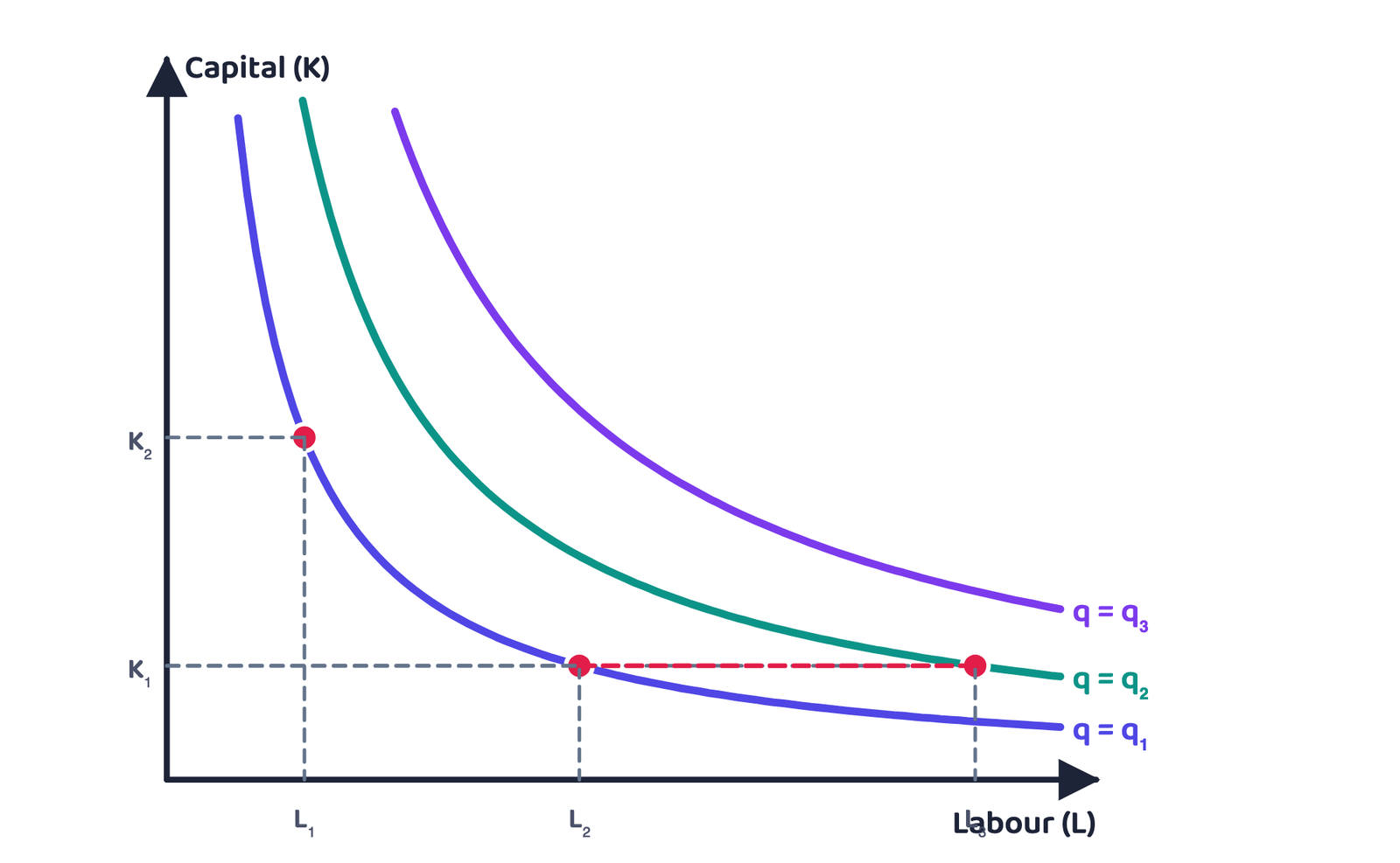
An isoquant is the set of all possible combinations of the two inputs that yield the same maximum possible level of output. Each isoquant represents a particular level of output and is labelled with that output.
- It is like the indifference curve of Chapter 2; an alternative way of representing the production function
- In Table 3.1, 10 units can be produced in three ways: (4L, 1K), (2L, 2K), (1L, 4K); all three lie on the isoquant q = 10
- On the isoquant q = 50: (6L, 3K), (4L, 4K), (3L, 6K)
- Diagram: L on the X axis, K on the Y axis; (L1, K2) and (L2, K1) give the same output q1; fixing capital at K1 and raising labour to L3 reaches the higher isoquant q2
- Negative slope: when marginal products are positive, with more of one input the same output can be produced only with less of the other
4 The short run and the long run
In the short run, at least one of the factors (labour or capital) cannot be varied and remains fixed. To vary output, the firm can vary only the other factor.
The factor that remains fixed in the short run is the fixed factor; the factor the firm can vary is the variable factor.
In the long run, all factors of production can be varied; the firm may vary both inputs simultaneously, so there is no fixed factor.
Short run
- At least one factor fixed
- Both fixed and variable factors
- Output changes only by changing the variable factor
- Fixed costs exist
- Example: in Table 3.1 with capital fixed at 4 units, the capital = 4 column
Long run
- All factors variable
- No fixed factor
- The firm can change all inputs together
- No fixed costs
- For a given process, generally a longer period than the short run
It is not advisable to define the short run and the long run in terms of days, months or years. The long run differs from one production process to another. The test is only this: can all the inputs be varied or not.
5 Total product, average product and marginal product
5.1 Total product
If we vary a single input and keep all other inputs constant, the relationship between the variable input and output is the total product (TP) of the variable input. It is also called the total return or total physical product of the variable input.
In Table 3.1 fix capital at 4 units and move down the capital = 4 column: this is the total product of labour (second column of Table 3.2).
5.2 Average product
Average product (AP) is output per unit of the variable input: (3.2)
5.3 Marginal product
The marginal product (MP) of an input is the change in output per unit of change in the input when all other inputs are held constant: (3.3)
Example: when L changes from 1 to 2, TP changes from 10 to 24; change in TP = 24 − 10 = 14, change in L = 1, so the MP of the 2nd unit of labour = 14/1 = 14
Table 3.2: Total Product, Marginal Product and Average Product (capital fixed at 4)
| Labour (L) | TP | MPL | APL |
|---|---|---|---|
| 0 | 0 | – | – |
| 1 | 10 | 10 | 10 |
| 2 | 24 | 14 | 12 |
| 3 | 40 | 16 | 13.33 |
| 4 | 50 | 10 | 12.5 |
| 5 | 56 | 6 | 11.2 |
| 6 | 57 | 1 | 9.5 |
- Inputs cannot take negative values, so marginal product is undefined at zero input
- TP = sum of marginal products: adding the MP of every unit up to a level gives TP at that level. Check: 10 + 14 + 16 + 10 + 6 + 1 = 57
- AP = average of the marginal products: at L = 3, (10 + 14 + 16) ÷ 3 = 40 ÷ 3 = 13.33
- Average and marginal products are also called the average and marginal returns to the variable input
Given
AP = 10 at L = 4, AP = 12 at L = 5
To find
MP of the 5th unit
- Formula: (½)
- TP at L = 4 = 10 × 4 = 40; TP at L = 5 = 12 × 5 = 60 (1)
- 20 units (½)
- Meaning: MP (20) is above the previous AP (10), which is why AP rose from 10 to 12
- Taking TP ÷ L as MP is wrong; that is AP. MP uses the change in TP
- Adding up APs to get TP is wrong; TP = AP × L. To get TP from MPs you add the MPs
- Writing MP = 0 at L = 0 is wrong; it is undefined
6 The law of diminishing marginal product and the law of variable proportions
- In Table 3.2, TP rises as labour rises, but not at a constant rate; the rate at which TP rises is shown by MP
- MP first rises (up to 3 units of labour: 10, 14, 16) and then falls (10, 6, 1)
The law of variable proportions (or the law of diminishing marginal product): the marginal product of a factor input initially rises with its employment level, but after reaching a certain level of employment, it starts falling.
Factor proportions represent the ratio in which the two inputs are combined to produce output.
- Take Table 3.2 as the output of a farmer with 4 hectares of land who can choose how much labour to use
- With only 1 worker there is too much land for one worker to cultivate alone
- As workers increase, labour per unit of land rises and each worker adds proportionally more to total output: MP rises
- When the fourth worker is hired, the land begins to get crowded; each worker has too little land to work efficiently, so each extra worker adds proportionally less: MP starts falling (16 to 10)
7 Returns to a factor: the three phases of the law of variable proportions
The CBSE curriculum lists “Returns to a Factor”. The CBSE Supplementary Reading Material explains it in three phases (phase 1, 2, 3) of TP and MP; the last column of the table gives the names these phases commonly go by:
| Phase | MP | TP | Name |
|---|---|---|---|
| Phase I | MP rises | TP rises at an increasing rate (curve convex from below) | increasing returns to a factor |
| Phase II | MP falls but stays positive | TP rises at a diminishing rate; TP is maximum where MP = 0 | diminishing returns to a factor |
| Phase III | MP negative | TP falls | negative returns to a factor |
Capital is fixed and labour is increased:
| L | 1 | 2 | 3 | 4 | 5 | 6 | 7 | 8 |
|---|---|---|---|---|---|---|---|---|
| TP | 8 | 20 | 36 | 48 | 56 | 60 | 60 | 56 |
| MP = TPL − TPL−1 | 8 | 12 | 16 | 12 | 8 | 4 | 0 | −4 |
| AP = TP/L | 8 | 10 | 12 | 12 | 11.2 | 10 | 8.57 | 7 |
- Phase I: L = 1 to 3 (MP rises 8 → 12 → 16)
- Phase II: L = 4 to 7 (MP 12 → 8 → 4 → 0, falling but not negative); at L = 7, MP = 0 and TP stays at its maximum of 60
- Phase III: L = 8 (MP = −4, TP falls from 60 to 56)
- Note: at L = 4, MP = AP = 12, and this is where AP is at its maximum (12)
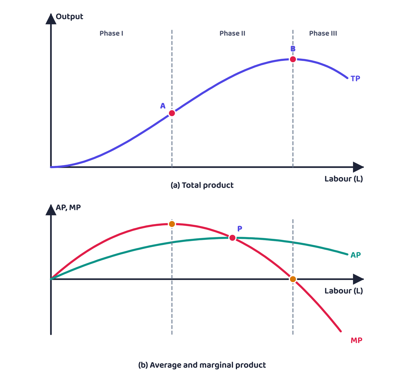
In the diagram, A is where TP rises fastest (MP is at its maximum); after A, TP rises at a diminishing rate. At B TP is maximum, and at exactly that L, MP is zero. At P, MP cuts AP from above, where AP is maximum.
8 Shapes of the TP, MP and AP curves
- TP curve (book Fig 3.1): raising one input with others constant raises output, so the TP curve in the input-output plane is positively sloped. Labour on the horizontal axis, output on the vertical axis; with L units of labour the firm can at most produce q1
- The book’s positive slope is the range where MP is positive; the supplement’s phase III (MP negative) adds the falling part of TP beyond it
- MP curve: by the law of variable proportions MP first rises and then falls, so the MP curve is an inverse ‘U’ (Fig 3.2)
- AP curve: for the first unit MP = AP. As MP rises, AP also rises, but less than MP. Even after MP starts falling, AP keeps rising as long as MP > AP. Once MP falls below AP, AP also falls. So the AP curve is also an inverse ‘U’
| Situation | AP | MP compared with AP |
|---|---|---|
| AP rising (left of AP’s maximum) | rising | MP > AP |
| AP at its maximum (at L in book Fig 3.2) | peak | MP = AP |
| AP falling (to the right) | falling | MP < AP |
The MP curve cuts the AP curve from above at the maximum point of AP. Reason: AP can rise only if MP is above AP, and AP falls only when MP is below AP.
- “Once MP starts falling, AP falls too” is wrong; AP rises as long as MP > AP (in Figure 2, MP peaks at A’s level of labour, L = 4, yet AP keeps rising until P, at L = 6)
- “MP cuts AP from below” is wrong; for product curves MP cuts from above (for cost curves MC cuts from below)
9 Returns to scale (Not in CBSE 2026-27 syllabus)
The law of variable proportions arises because factor proportions change when one factor is held constant and the other is increased. Both factors can change only in the long run. One special case: both factors increased in the same proportion (factors scaled up).
Constant returns to scale (CRS)
A proportional increase in all inputs raises output by the same proportion. Inputs doubled ⇒ output doubled
Increasing returns to scale (IRS)
Output rises by a larger proportion. Inputs doubled ⇒ output more than doubled
Decreasing returns to scale (DRS)
Output rises by a smaller proportion. Inputs doubled ⇒ output less than doubled
; increase both factors t times ():
Cobb-Douglas production function
, where α and β are constants, is called a Cobb-Douglas production function.
- : 0.6 + 0.4 = 1 ⇒ CRS
- : 0.7 + 0.5 = 1.2 > 1 ⇒ IRS
- : 0.3 + 0.4 = 0.7 < 1 ⇒ DRS
- : 2 + 2 = 4 ⇒ IRS; at L = 5, K = 2, Q = 2 × 25 × 4 = 200, and at L = 10, K = 4, Q = 3,200 = 16 × 200 (inputs doubled, output 24 = 16 times)
| Basis | Returns to a factor (variable proportions) | Returns to scale |
|---|---|---|
| Period | Short run | Long run |
| Factors that change | Only one; the rest fixed | All, in the same proportion |
| Factor proportions | Change | Stay the same |
| Measured by | Rise or fall of MP | Proportionate change in output |
10 Costs and the cost function
- A given output can usually be produced with more than one input combination. In Table 3.1, 50 units can be produced by three: (L = 6, K = 3), (L = 4, K = 4), (L = 3, K = 6)
- With input prices given, the firm chooses the combination that is least expensive: for every level of output, the least cost input combination
The cost function describes the least cost of producing each level of output, given the prices of factors of production and technology.
Explicit cost
- Actual money expenditure on inputs (definition from the CBSE supplement)
- For instance wages, payment for raw material, rent of a hired machine
Implicit cost (CBSE supplement)
- Estimated money value of inputs supplied by the owners, including normal profit
- For example the owner’s estimated salary, estimated interest on own money invested, estimated rent of the owner’s building
Normal profit is the minimum profit the owners must get in the long run to stay in the current business rather than shift to the next best alternative.
11 Short run costs: TFC, TVC and TC
Total fixed cost (TFC) is the cost a firm incurs to employ the fixed inputs in the short run. Whatever the output, this cost remains fixed (even at zero output).
Total variable cost (TVC) is the cost a firm incurs to employ the variable inputs. More output needs more variable inputs, so TVC rises with output; at zero output TVC is zero.
Total cost (TC) is the sum of fixed and variable costs: (3.6)
Table 3.3: Various Concepts of Costs (all costs in Rs)
| Output (q) | TFC | TVC | TC | AFC | AVC | SAC | SMC |
|---|---|---|---|---|---|---|---|
| 0 | 20 | 0 | 20 | – | – | – | – |
| 1 | 20 | 10 | 30 | 20 | 10 | 30 | 10 |
| 2 | 20 | 18 | 38 | 10 | 9 | 19 | 8 |
| 3 | 20 | 24 | 44 | 6.67 | 8 | 14.67 | 6 |
| 4 | 20 | 29 | 49 | 5 | 7.25 | 12.25 | 5 |
| 5 | 20 | 33 | 53 | 4 | 6.6 | 10.6 | 4 |
| 6 | 20 | 39 | 59 | 3.33 | 6.5 | 9.83 | 6 |
| 7 | 20 | 47 | 67 | 2.86 | 6.7 | 9.57 | 8 |
| 8 | 20 | 60 | 80 | 2.5 | 7.5 | 10 | 13 |
| 9 | 20 | 75 | 95 | 2.22 | 8.33 | 10.55 | 15 |
| 10 | 20 | 95 | 115 | 2 | 9.5 | 11.5 | 20 |
Values as in the book’s Table 3.3. Worked to two decimals, AVC at q = 7 is 47/7 = 6.71 and SAC at q = 9 is 95/9 = 10.56.
- TFC = ₹20 at every output; at zero output TC = TFC = ₹20
- For 1 unit, TVC = ₹10 and TC = ₹30; for 2 units, TVC = ₹18 and TC = ₹38
- TFC is fixed, so every change in TC comes only from the change in TVC
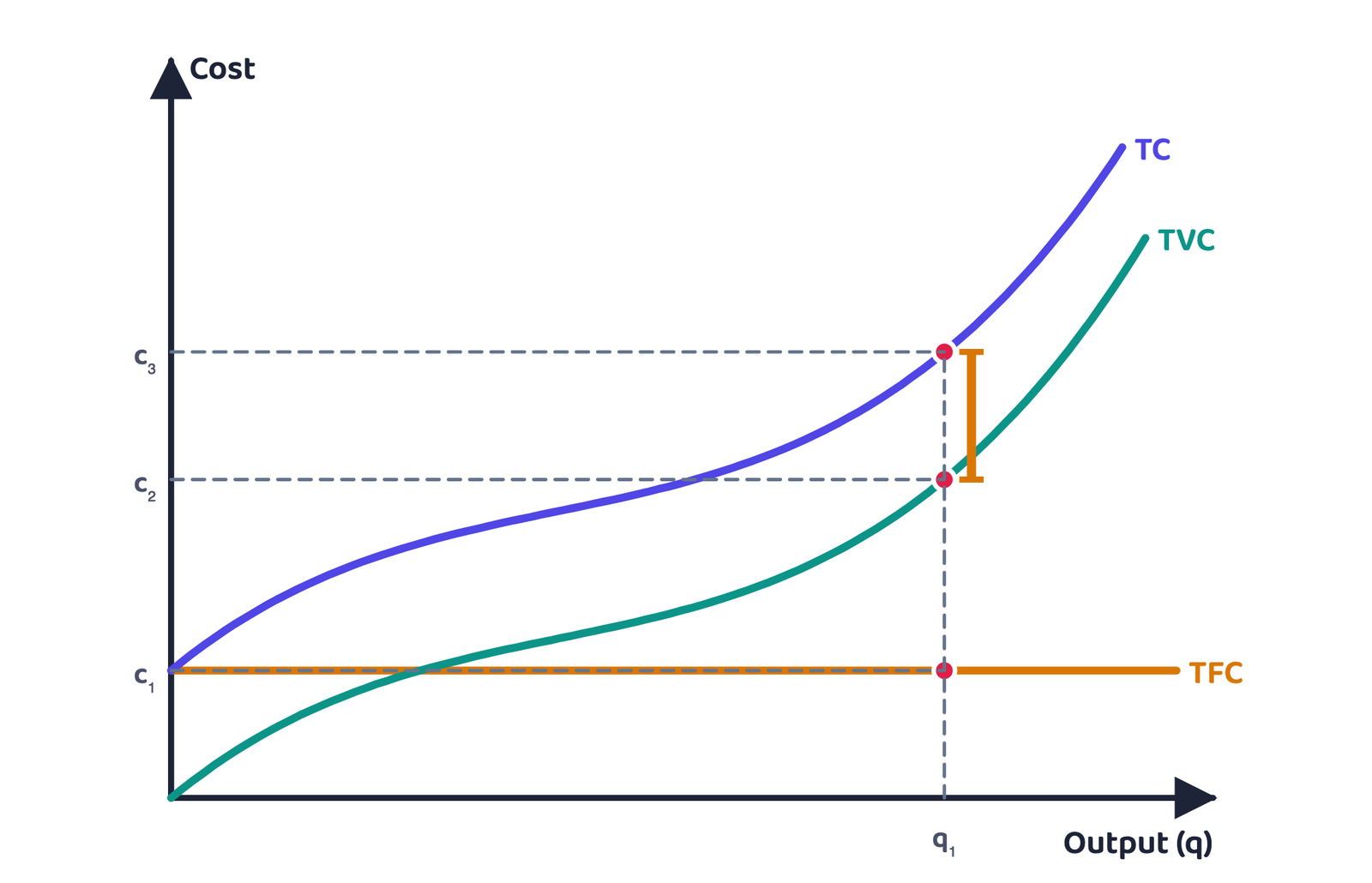
- TFC curve: independent of output, so a horizontal straight line cutting the cost axis at c1
- TVC curve: starts at the origin and rises; at q1, TVC = c2
- TC curve: the vertical sum of TFC and TVC; at q1, TC = c3. It starts at the height of TFC (c1) and runs exactly c1 above TVC, with the same shape
12 Average costs and marginal cost
Short run average cost (SAC) is total cost per unit of output: (3.7)
Average variable cost (AVC) is total variable cost per unit of output: (3.8)
Average fixed cost (AFC) is total fixed cost per unit of output: (3.9)
Short run marginal cost (SMC) is the change in total cost per unit of change in output: (3.11)
Book example (q = 5): change in TC = 53 − 49 = 4, change in q = 1, SMC = 4/1 = ₹4 (3.12)
- At zero output SAC, AVC, AFC and SMC are all undefined
- For the first unit: AFC = ₹20, AVC = ₹10, and their sum SAC = ₹30; for the first unit SMC = AVC = ₹10
- Fixed cost cannot change in the short run, so marginal cost = the increase in TVC from producing one extra unit (CBSE supplement: TFC is the same in both terms and cancels)
- Sum of marginal costs = TVC: in Table 3.3, 10 + 8 + 6 + 5 + 4 + 6 + 8 + 13 + 15 + 20 = 95 = TVC at q = 10
- So AVC = the average of all marginal costs up to that level; and the area under the SMC curve up to an output is the TVC up to that output
Given
TFC = ₹60; TVC (q = 1 to 6): 40, 70, 90, 120, 160, 216
To find
TC, AFC, AVC, AC, MC
| q | TVC | TC = TFC + TVC | AFC = 60/q | AVC = TVC/q | AC = TC/q | MC = ΔTC |
|---|---|---|---|---|---|---|
| 0 | 0 | 60 | – | – | – | – |
| 1 | 40 | 100 | 60 | 40 | 100 | 40 |
| 2 | 70 | 130 | 30 | 35 | 65 | 30 |
| 3 | 90 | 150 | 20 | 30 | 50 | 20 |
| 4 | 120 | 180 | 15 | 30 | 45 | 30 |
| 5 | 160 | 220 | 12 | 32 | 44 | 40 |
| 6 | 216 | 276 | 10 | 36 | 46 | 56 |
- Check: in every row AFC + AVC = AC (e.g. q = 5: 12 + 32 = 44) (½)
- At q = 4, MC = AVC = ₹30, where AVC is at its minimum (½)
- At q = 5, MC (40) < previous AC (45), so AC falls to 44; at q = 6, MC (56) > AC (44), so AC rises to 46 (½)
- Meaning: AC is lowest at q = 5 and AVC at q = 3-4
- To get TFC from a TC table, take the TC at q = 0; that is TFC (and it is the same at every level)
- AFC × q = TFC, but AVC × q = TVC; mixing them up is wrong
- Finding MC as TC/q is wrong (that is AC); MC is the difference between two successive TCs
- “TFC affects MC” is wrong; a change in TFC changes AFC and AC, not MC or AVC
13 Shapes of the short run cost curves
13.1 The AFC curve
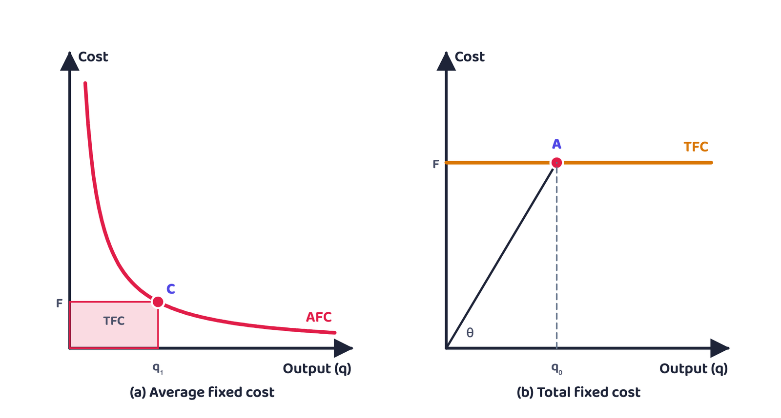
- AFC = TFC/q with TFC constant, so as q increases AFC keeps falling
- When output is very close to zero, AFC is arbitrarily large; as output moves towards infinity, AFC moves towards zero, but never reaches it
- The AFC curve is a rectangular hyperbola: multiplying any q by its AFC always gives the same constant (TFC)
- Fig 3.4: at q1, AFC = OF; = area of rectangle OFCq1
- Fig 3.5: AFC from the TFC curve: point A on the TFC curve at q0; if ∠AOq0 = θ, then
13.2 Why the SMC curve is U-shaped
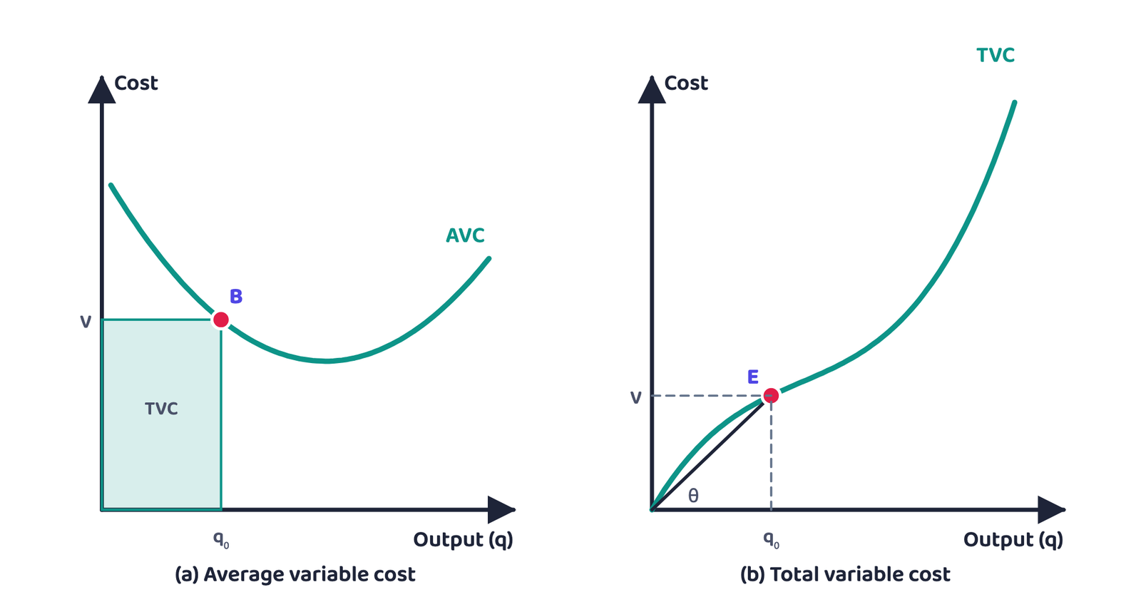
13.3 The AVC curve
- For the first unit SMC = AVC, so both curves start from the same point
- As output rises SMC falls; AVC, being the average of marginal costs, also falls, but less than SMC
- Even when SMC starts rising, AVC keeps falling as long as SMC < AVC; once SMC rises above AVC, AVC starts rising. So the AVC curve is U-shaped
- Fig 3.6: at q0, AVC = OV; = area of rectangle OVBq0
- Fig 3.7: AVC from the TVC curve: point E on the TVC curve at q0, OV = TVC; if ∠EOq0 = θ, then
13.4 The SAC curve
- SAC = AVC + AFC. At first both AVC and AFC fall, so SAC falls
- After a certain output AVC starts rising, but AFC keeps falling. At first the fall in AFC is greater than the rise in AVC, so SAC still falls
- After a certain level the rise in AVC becomes larger than the fall in AFC; from then on SAC rises. So the SAC curve is U-shaped
- SAC lies above AVC; the vertical gap between them = AFC (which keeps shrinking, so the two curves come closer but never meet)
- The minimum of SAC lies to the right of the minimum of AVC
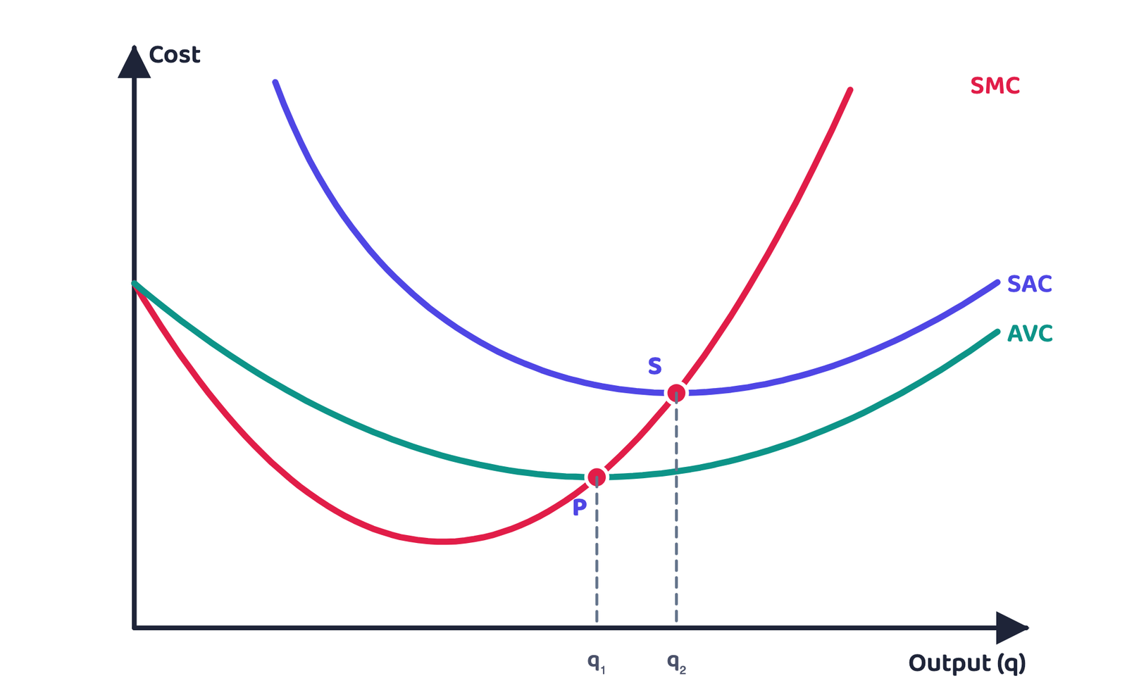
The SMC curve cuts the AVC curve from below at the minimum point of AVC (P) and cuts the SAC curve from below at the minimum point of SAC (S). Reason: as long as an average is falling, the marginal must be below it; when the average is rising, the marginal must be above it.
In Fig 3.8, P is at output q1 and S at output q2; to the left of q1 and q2 the marginal is below the average, to the right it is above.
13.5 The arithmetic relation between MC and AC (CBSE supplement)
| Output | TC (₹) | MC (₹) | AC (₹) | Relation |
|---|---|---|---|---|
| 1 | 60 | 60 | 60 | First unit: MC = AC |
| 2 | 110 | 50 | 55 | MC < AC ⇒ AC falls |
| 3 | 162 | 52 | 54 | MC < AC ⇒ AC falls (even though MC rose) |
| 4 | 216 | 54 | 54 | MC = AC ⇒ AC constant |
| 5 | 275 | 59 | 55 | MC > AC ⇒ AC rises |
- This relation holds for the average and marginal values of any variable (revenue, product and so on)
- A rising MC does not mean a rising AC: at q = 3, MC rose from 50 to 52 but AC fell from 55 to 54
- “SMC can cut AVC at any point” is wrong; always at the minimum of AVC, from below
- Drawing AFC as a U is wrong; it is a continuously falling rectangular hyperbola that never touches the X axis
- Letting SAC and AVC meet is wrong; the gap between them, AFC, is never zero
14 Long run costs (Not in CBSE 2026-27 syllabus)
- In the long run all inputs are variable, so there are no fixed costs; total cost and total variable cost coincide
- Long run average cost: (3.13)
- Long run marginal cost: raising output from q1 − 1 to q1, (3.14)
- As in the short run, the sum of all marginal costs up to an output gives total cost at that output
| Returns to scale | Inputs needed to raise output by a proportion | Cost | LRAC |
|---|---|---|---|
| IRS | Less than that proportion (double output with less than double inputs) | rises by a smaller proportion | falls |
| CRS | The same proportion | the same proportion | constant |
| DRS | More than that proportion | a larger proportion | rises |
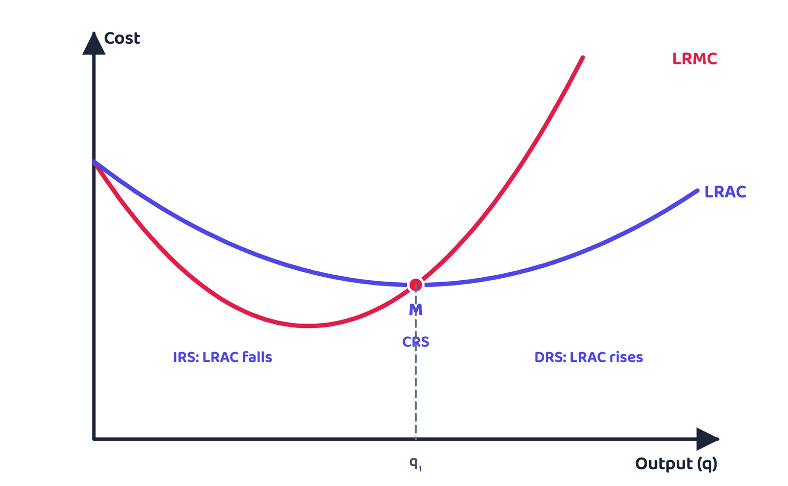
- It is argued that a typical firm shows IRS at the initial level of production, then CRS, then DRS; so the LRAC curve is U-shaped
- The downward part corresponds to IRS and the rising part to DRS; at the minimum of LRAC, CRS is observed
- For the first unit LRMC = LRAC; while LRAC falls LRMC < LRAC, and while LRAC rises LRMC > LRAC. So LRMC is also U-shaped and cuts LRAC from below at its minimum point M (Fig 3.9)
- LRAC is minimum at q1: to the left of q1 LRMC < LRAC, to the right LRMC > LRAC
15 Key formulas and difference tables
| Basis | Fixed cost | Variable cost |
|---|---|---|
| Meaning | Cost of fixed inputs | Cost of variable inputs |
| Relation to output | Independent of output | Rises with output |
| At zero output | Positive (TC = TFC) | Zero |
| Period | Short run only | Short run and long run |
| Curves | Horizontal line (TFC); rectangular hyperbola (AFC) | Rises from origin (TVC); U (AVC) |
| Relation | Product curves | Cost curves |
|---|---|---|
| Shape | AP, MP inverse U | AVC, SAC, SMC U |
| Crossing | MP cuts AP at its maximum from above | SMC cuts AVC and SAC at their minimum from below |
| Sum | Sum of MPs = TP | Sum of SMCs = TVC |
| Reason | Law of variable proportions | The same law in reverse (MP rises, so MC falls) |
16 All definitions together
- The production function gives maximum output; for a given technology, efficient use only
- Short run: at least one factor fixed; long run: all variable; not defined in days or years
- AP = TP/L, MP = ΔTP/ΔL; TP = sum of MPs; in Table 3.2, TP 57 = 10 + 14 + 16 + 10 + 6 + 1
- MP first rises then falls: law of variable proportions (cause: changing factor proportions, crowding)
- Three phases: MP rising / MP falling but positive / MP negative; TP is maximum where MP = 0
- MP and AP are inverse U; MP cuts AP from above at AP’s maximum
- TC = TFC + TVC; SAC = AFC + AVC; SMC = ΔTC = ΔTVC; TVC = sum of SMCs
- AFC is a rectangular hyperbola (AFC × q = TFC); TFC is a horizontal line
- SMC, AVC, SAC are U; SMC cuts both at their minima from below; SAC’s minimum is to the right of AVC’s
- CRS/IRS/DRS: inputs doubled ⇒ output doubled / more / less; Cobb-Douglas: compare α + β with 1
- No fixed cost in the long run; LRAC U (IRS, CRS, DRS); LRMC cuts LRAC at M from below
- Can I build AP and MP from TP, TP from AP, and TP from MP?
- Can I fill TFC, TVC, AFC, AVC, SAC and SMC from a TC table?
- Can I draw TP, AP and MP with all three phases?
- Can I draw SMC, AVC and SAC with points P and S and write why SMC cuts them there?
- Can I explain AFC with the rectangular hyperbola and the rectangle OFCq1?
- Can I tell the law of variable proportions apart from returns to scale?